


Next: Results Up: FINDING REARRANGEMENT PATHWAYS Previous: L-BFGS Minimiser Contents
Single-ended methods use only the function and its derivatives to search for a transition state from the starting point (the initial guess). Since a transition state is a local maximum in one direction but a minimum in all the others it is not generally possible to use standard minimisation methods for this purpose. Newton-type optimisation methods are based on approximating the objective function locally by a quadratic model and then minimising that function approximately using, for example, the Newton-Raphson (NR) approach [31]. However, the NR algorithm can converge to a stationary point of any index [130]. To converge to a transition state the algorithm may need to start from a geometry at which the Hessian has exactly one negative eigenvalue and the corresponding eigenvector is at least roughly parallel to the reaction coordinate. Locating such a point can be a difficult task and several methods have been developed that help to increase the basins of attraction of transition states, which gives more freedom in choosing the starting geometry [9,22,24,19].
The most widely used single-ended transition state search method is eigenvector-following (EF). In it simplest form it requires diagonalisation of the Hessian matrix [12,14,13,15]. For larger systems it is advantageous to use hybrid EF methods that avoid either calculating the Hessian or diagonalising it [22,133,23,8].
We start by reviewing the theory behind the Newton-Raphson methods. Solving the eigenvalue problem
 | (4.21) |
yields the matrix  , the columns of which are the eigenvectors
  , and the diagonal matrix
  , with eigenvalues
  on the diagonal. The matrix defines a unitary transformation to a new orthogonal basis
  , in which the original Hessian matrix
  is diagonal
 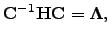 | (4.22) |
so that Equation 2.13 is simplified to  | (4.23) |
where  is the gradient vector in the new basis, which is related to the original gradient vector
  as
as  | (4.24) |
because of the unitarity of  | (4.25) |
The unnormalised search direction  is defined similarly.
 After taking a step of length  in the direction
  , as prescribed by Equation 2.23, the energy changes by
 | (4.26) |
provided our quadratic approximation to  is perfect. In general
  and terms in Equation 2.26 with
  and
and  increase and decrease the energy, respectively. For isolated molecules and bulk models with periodic boundary conditions the Hessian matrix is singular: there are three zero eigenvalues that correspond to overall translations. Non-linear isolated molecules have three additional zero eigenvalues due to rotations. Luckily, in all cases for which
  the analytic form of the corresponding eigenvectors is known so the eigenvalue shifting procedure could be applied:
 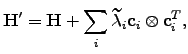 | (4.27) |
where  are the new eigenvalues. In this work all the zero eigenvalues were shifted by the same amount (
 ). As a result,
  and problems with applying Equation 2.23 do not arise.
 The analytic forms of the 's corresponding to translations along the  ,
,  and
and  directions are
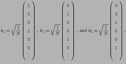 | (4.28) |
respectively. The eigenvector that corresponds to rotation about the axis by a small angle  can be obtained as
 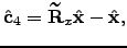 | (4.29) |
where  is a normalised
  -dimensional vector describing the position before the rotation, and
  is Maclaurin series expansion of the -dimensional rotation matrix [134]
  with respect to a small angle truncated to the second order. The displacement vectors due to infinitesimal rotation about the , and axes are therefore
  | (4.30) |
respectively. If started from a point at which the Hessian matrix has  negative eigenvalues, the NR method is expected to converge to a stationary point of index . However, the step taking procedure may change the index as optimisation proceeds.
Introducing Lagrange multipliers allows a stationary point of specified index to be located. Consider a Lagrangian function
![$\displaystyle L=-V'({\bf x}'_0)-\sum_{\alpha=1}^{3N}\left[ g'_\alpha({\bf x}'_0...
...alpha\, {p'}_\alpha^2 - {1\over2} \mu_\alpha({p'}_\alpha^2-c_\alpha^2) \right],$](img412.png) | (4.31) |
where a separate Lagrange multiplier  is used for every eigendirection
  ,
,  is a constraint on the step
  ,
,  is the th eigenvalue of
  , which is defined in Equation 2.27, and
  is the point about which the potential energy function
  was expanded. Primes, as before, denote that components are expressed in the orthogonal basis. Differentiating Equation 2.31 with respect to and using the condition for a stationary point the optimal step can be obtained:
  | (4.32) |
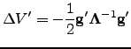
The predicted energy change corresponding to this step is  | (4.33) |
We have some freedom in choosing the Lagrange multipliers as long as for the eigendirections for which an uphill (downhill) step is to be taken  (
(  ). The following choice of Lagrange multipliers allows the recovery of the Newton-Raphson step in the vicinity of a stationary point [9]:
  | (4.34) |
with the plus sign for an uphill step, and the minus sign for a downhill step. In cases when Hessian diagonalisation is impossible or undesirable the smallest eigenvalue and a corresponding eigenvector can be found using an iterative method [135].
Next: Results Up: FINDING REARRANGEMENT PATHWAYS Previous: L-BFGS Minimiser Contents Semen A Trygubenko 2006-04-10