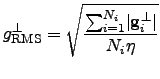
Specifically, it is possible to quench velocities right after advancing the system using Equation 2.14, at the half-step in the velocity evaluation (quenching intermediate velocities at time ![]() ) using either the old or new gradient [Equation 2.15], or after completion of the velocity update. In Figure 2.4 we present results for the stability of NEB/QVV as a function of the force constant parameter for three of these quenching approaches. We will refer to an NEB optimisation as stable for a certain combination of parameters (e.g. time integration step, number of images) if the NEB steadily converges to a well-defined path and/or stays in its proximity until the maximal number of iterations is reached or the convergence criterion is satisfied.
) using either the old or new gradient [Equation 2.15], or after completion of the velocity update. In Figure 2.4 we present results for the stability of NEB/QVV as a function of the force constant parameter for three of these quenching approaches. We will refer to an NEB optimisation as stable for a certain combination of parameters (e.g. time integration step, number of images) if the NEB steadily converges to a well-defined path and/or stays in its proximity until the maximal number of iterations is reached or the convergence criterion is satisfied.
We have performed some of the tests on the Müller-Brown (MB) two-dimensional surface [25]. This widely used surface does not present a very challenging or realistic test case, but if an algorithm does not behave well for this system it is unlikely to be useful. MB potential is defined as a sum of four terms, each of which takes the form
![$\displaystyle V_i(x,y) = \alpha \exp \left[ a \left(x - x_0\right)^2 + b \left(x - x_0\right) \left(y - y_0\right) + c \left(y - y_0\right)^2 \right],$](img425.png) | (4.35) |
![\begin{psfrags}
\psfrag{-1.5} [Bc][Bc]{$-1.5$}
\psfrag{-1.0} [Bc][Bc]{$-1.0$...
... \centerline{\includegraphics[width=.50\textheight]{dneb/MB.eps}}
\end{psfrags}](img434.png) |
Figure 2.4 shows the results of several thousand optimisations for a 17-image band with the MB two-dimensional potential [25] using QVV minimisation and a time step of ![]() (consistent units) for different values of
(consistent units) for different values of ![]() .
.
![\begin{psfrags}
\psfrag{k} [Bc][Bc]{$k_{spr}/10^3$}
\psfrag{l} [Bc][Bc]{$\el...
...
\centerline{\includegraphics[width=.40\textheight]{dneb/q.eps}}
\end{psfrags}](img435.png) |
It seems natural to remove the velocity component perpendicular to the gradient at the current point when the geometry ![]() , gradient
, gradient ![]() and velocity
and velocity ![]()
![]() are available, i.e.
are available, i.e.
From Figure 2.4 (a) we see that the best approach is to quench the velocity after the coordinate update. The optimisation is then stable for a wide range of force constant values, and the images on the resulting pathway are evenly distributed. In this quenching formulation the velocity response to a new gradient direction is retarded by one step in coordinate space: the step is still taken in the direction ![]()
![]() but the corresponding velocity component is removed. To implement this slow-response QVV (SQVV) it is necessary to modify the VV algorithm described in Section 2.5.1 by inserting Equation 2.37 in between the two stages described by Equation 2.14 and Equation 2.15.
but the corresponding velocity component is removed. To implement this slow-response QVV (SQVV) it is necessary to modify the VV algorithm described in Section 2.5.1 by inserting Equation 2.37 in between the two stages described by Equation 2.14 and Equation 2.15.
The second-best approach after SQVV is to quench the velocity at midstep ![]() using the new gradient. On average, this algorithm takes twice as long to converge the NEB to a given RMS gradient tolerance compared to SQVV. However, the method is stable for the same range of spring force constant values and produces a pathway in which the images are equispaced more accurately than the other formulations [see Figure 2.4 (b)].
using the new gradient. On average, this algorithm takes twice as long to converge the NEB to a given RMS gradient tolerance compared to SQVV. However, the method is stable for the same range of spring force constant values and produces a pathway in which the images are equispaced more accurately than the other formulations [see Figure 2.4 (b)].
The least successful of the three QVV schemes considered involves quenching velocities at mid-step using the gradient from the previous iteration (stars in Figure 2.4). Even though the number of iterations required is roughly comparable to that obtained by quenching using the new gradient, it has the smallest range of values for the force constant where it is stable. Some current implementations of NEB [137,136] (intended for use in combination with electronic structure codes) use this type of quenching in their QVV implementation.
We have also conducted analogous calculations for more complicated systems such as permutational rearrangements of Lennard-Jones clusters. The results are omitted for brevity, but agree with the conclusions drawn from the simpler 2D model described above. The same is true for the choice of force constant investigated in the following section.