As test cases for this algorithm we have considered various degenerate rearrangements of LJ![]() , LJ
, LJ![]() , LJ
, LJ![]() and LJ
and LJ![]() . (A degenerate rearrangement is one that links permutational isomers of the same structure [9,148].) In addition, we have considered rearrangements that link second lowest-energy structure with a global minimum for LJ
. (A degenerate rearrangement is one that links permutational isomers of the same structure [9,148].) In addition, we have considered rearrangements that link second lowest-energy structure with a global minimum for LJ![]() and LJ
and LJ![]() clusters. The PES's of LJ
clusters. The PES's of LJ![]() and LJ
and LJ![]() have been analysed in a number of previous studies [150,113,149,151], and are known to exhibit a double-funnel morphology: for both clusters the two lowest-energy minima are structurally distinct and well separated in configuration space. This makes them useful benchmarks for the above connection algorithm. Figure 2.9 depicts the energy profiles obtained using the revised connection algorithm for rearrangements between the two lowest minima of each cluster. In each case we have considered two distinct paths that link different permutational isomers of the minima in question, and these were chosen to be the permutations that give the shortest Euclidean distances. These paths will be identified using the distance between the two endpoints; for example, in the case of LJ
have been analysed in a number of previous studies [150,113,149,151], and are known to exhibit a double-funnel morphology: for both clusters the two lowest-energy minima are structurally distinct and well separated in configuration space. This makes them useful benchmarks for the above connection algorithm. Figure 2.9 depicts the energy profiles obtained using the revised connection algorithm for rearrangements between the two lowest minima of each cluster. In each case we have considered two distinct paths that link different permutational isomers of the minima in question, and these were chosen to be the permutations that give the shortest Euclidean distances. These paths will be identified using the distance between the two endpoints; for example, in the case of LJ![]() we have paths LJ
we have paths LJ![]()
![]() and LJ
and LJ![]()
![]() , where
, where ![]() is the pair equilibrium separation for the LJ potential.
is the pair equilibrium separation for the LJ potential.
![\begin{psfrags}
\psfrag{5} [bc][bc]{$5$}
\psfrag{10} [bc][bc]{$10$}
\psfra...
...centerline{\includegraphics[width=.8\textheight]{dneb/tests.eps}}
\end{psfrags}](img468.png) |
For each calculation we used the following settings: the initial image density was set to 10, the iteration density to 30, and the maximum number of attempts to connect any pair of minima was limited to three. If a connection failed for a particular pair of minima then up to two more attempts were allowed before moving to the pair with the next smallest separation. For the second and third attempts the number of images was increased by ![]() each time. The maximum number of EF optimisation steps was set to
each time. The maximum number of EF optimisation steps was set to ![]() with an RMS force convergence criterion of
with an RMS force convergence criterion of ![]() . In Figure 2.9 every panel is labelled with the separation between the endpoints, the number of transition states in the final pathway, the number of DNEB runs required, and the total number of gradient calls.
. In Figure 2.9 every panel is labelled with the separation between the endpoints, the number of transition states in the final pathway, the number of DNEB runs required, and the total number of gradient calls.
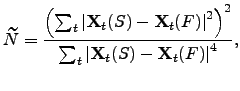
Individual pathways involving a single transition state have been characterised using indices [152] such as
We have found that it is usually easier to locate good transition state candidates for a multi-step path if the stationary points are separated by roughly equal distances, in terms of the integrated path length. Furthermore, it seems that more effort is needed to characterise a multi-step path when transition states involving very different path lengths are present. In such cases it is particularly beneficial to build up a complete path in stages. To further characterise this effect we introduce a path length asymmetry index ![]() defined as
defined as
 | (4.42) |
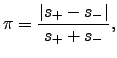
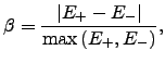
Barrier asymmetry also plays a role in the accuracy of the tangent estimate, the image density required to resolve particular regions of the path, and in our selection process for transition state candidates, which is based on the condition ![]() .[2] Unless there is no maximum in the profile, in which case we consider for transition state searching the highest energy image. To characterise this property we define a barrier asymmetry index,
.[2] Unless there is no maximum in the profile, in which case we consider for transition state searching the highest energy image. To characterise this property we define a barrier asymmetry index, ![]() , as
, as
 | (4.43) |
We note that the total number of gradient evaluations required to produce the above paths could be reduced significantly by optimising the DNEB parameters or the connection strategy in each case. However, our objective was to find parameters that give reasonable results for a range of test cases, without further intervention.