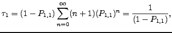
The KMC method can be used to generate a memoryless (Markovian) random walk and hence a set of trajectories connecting initial and final states in a DPS database. Many trajectories are necessary to collect appropriate statistics. Examples of pathway averages that are usually obtained with KMC are the mean path length and the mean first passage time. Here the KMC trajectory length is the number of states (local minima of the PES in the current context) that the walker encounters before reaching the final state. The first passage time is defined as the time that elapses before the walker reaches the final state. For a given KMC trajectory the first passage time is calculated as the sum of the mean waiting times in each of the states encountered.
Within the canonical Metropolis Monte Carlo approach a step is always taken if the proposed move lowers the energy, while steps that raise the energy are allowed with a probability that decreases with the energy difference between the current and proposed states [32]. An efficient way to propagate KMC trajectories was suggested by Bortz, Kalos, and Lebowitz (BKL) [190]. According to the BKL algorithm, a step is chosen in such a way that the ratios between transition probabilities of different events are preserved, but rejections are eliminated. Figure 4.1 explains this approach for a simple discrete-time Markov chain. The evolution of an ordinary KMC trajectory is monitored by the `time' parameter ![]() ,
, ![]() , which is incremented by one every time a transition from any state is made. The random walker is in state
, which is incremented by one every time a transition from any state is made. The random walker is in state ![]() at time
at time ![]() . The KMC trajectory is terminated whenever an absorbing state is encountered. As
. The KMC trajectory is terminated whenever an absorbing state is encountered. As ![]() approaches unity transitions out of state
approaches unity transitions out of state ![]() become rare. To ensure that every time a random number is generated (one of the most time consuming steps in a KMC calculation) a move is made to a neighbouring state we average over the transitions from state
become rare. To ensure that every time a random number is generated (one of the most time consuming steps in a KMC calculation) a move is made to a neighbouring state we average over the transitions from state ![]() to itself to obtain the Markov chain depicted in Figure 4.1 (b).
to itself to obtain the Markov chain depicted in Figure 4.1 (b).
![\begin{psfrags}
\psfrag{nav} [bc][bc]{$\tau_1$}
\psfrag{1} [bc][bc]{$1$}
\...
...g{B} [bc][bc]{(b)}
\centerline{\includegraphics{markov/BKL.eps}}
\end{psfrags}](img640.png) |
 | (6.2) |
 | (6.3) |
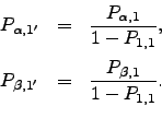
Similar ideas underlie the accelerated Monte Carlo algorithm suggested by Novotny [26]. According to this `Monte Carlo with absorbing Markov chains' (MCAMC) method, at every step a Markov matrix, ![]() , is formed, which describes the transitions in a subspace
, is formed, which describes the transitions in a subspace ![]() that contains the current state
that contains the current state ![]() , and a set of adjacent states that the random walker is likely to visit from
, and a set of adjacent states that the random walker is likely to visit from ![]() . A trajectory length,
. A trajectory length, ![]() , for escape from
, for escape from ![]() is obtained by bracketing a uniformly distributed random variable,
is obtained by bracketing a uniformly distributed random variable, ![]() , as
, as
![$\displaystyle \sum_{\beta} \left[{\bf P}^{n}\right]_{\beta,\alpha} < r \leqslant \sum_{\beta} \left[{\bf P}^{n-1}\right]_{\beta,\alpha}.$](img643.png) | (6.4) |
![$\displaystyle \left[{\bf R}{\bf P}^{n-1}\right]_{\gamma,\alpha}/ \sum_{\gamma} \left[{\bf R}{\bf P}^{n-1}\right]_{\gamma,\alpha},$](img645.png) | (6.5) |
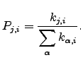
In chemical kinetics transitions out of a state are described using a Poisson process, which can be considered a continuous-time analogue of Bernoulli trials. The transition probabilities are determined from the rates of the underlying transitions as
 | (6.6) |
Given the exponential distribution of waiting times the mean waiting time in state ![]() before escape,
before escape, ![]() , is
, is ![]() and the variance of the waiting time is simply
and the variance of the waiting time is simply ![]() . Here
. Here ![]() is the rate constant for transitions from
is the rate constant for transitions from ![]() to
to ![]() . When the average of the distribution of times is the property of interest, and not the distribution of times itself, it is sufficient to increment the simulation time by the mean waiting time rather than by a value drawn from the appropriate distribution [9,205]. This modification to the original KMC formulation [207,206] reduces the cost of the method and accelerates the convergence of KMC averages without affecting the results.
. When the average of the distribution of times is the property of interest, and not the distribution of times itself, it is sufficient to increment the simulation time by the mean waiting time rather than by a value drawn from the appropriate distribution [9,205]. This modification to the original KMC formulation [207,206] reduces the cost of the method and accelerates the convergence of KMC averages without affecting the results.