


Next: KMC and DPS Averages Up: Introduction Previous: The Kinetic Monte Carlo Contents
Discrete Path Sampling
The result of a DPS simulation is a database of local minima and transition states from the PES [9,10,8]. To extract thermodynamic and kinetic properties from this database we require partition functions for the individual minima and rate constants,  , for the elementary transitions between adjacent minima
  and
and  . We usually employ harmonic densities of states and statistical rate theory to obtain these quantities, but these details are not important here. To analyse the global kinetics we further assume Markovian transitions between adjacent local minima, which produces a set of linear (master) equations that governs the evolution of the occupation probabilities towards equilibrium [196,189]
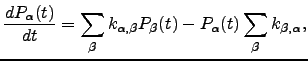 | (6.7) |
where  is the occupation probability of minimum at time
  .
. All the minima are classified into sets  ,
,  and
and  .When local equilibrium is assumed within the and sets we can write
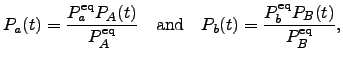 | (6.8) |
where 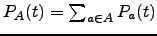 and
and 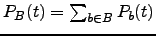 .If the steady-state approximation is applied to all the intervening states
 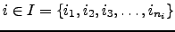 , so that
  | (6.9) |
then Equation 4.7 can be written as [9] 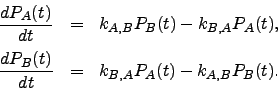 | (6.10) |
The rate constants  and
and  for forward and backward transitions between states and are the sums over all possible paths within the set of intervening minima of the products of the branching probabilities corresponding to the elementary transitions for each path:
 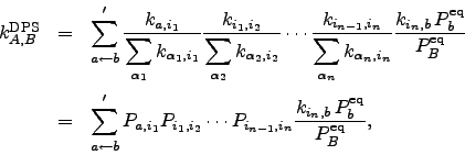 | (6.11) |
and similarly for [8]. The sum is over all paths that begin from a state  and end at a state
  , and the prime indicates that paths are not allowed to revisit states in . In previous contributions [133,10,197,8] this sum was evaluated using a weighted adjacency matrix multiplication (MM) method, which will be reviewed in Section 4.2.
Next: KMC and DPS Averages Up: Introduction Previous: The Kinetic Monte Carlo Contents Semen A Trygubenko 2006-04-10