We now show that the evaluation of the DPS sum in Equation 4.11 and the calculation of KMC averages are two closely related problems.
For KMC simulations we define sources and sinks that coincide with the set of initial states ![]() and final states
and final states ![]() , respectively.[1] Terminology taken from graph theory. In probability theory, state
, respectively.[1] Terminology taken from graph theory. In probability theory, state ![]() is called absorbing if
is called absorbing if ![]() , which coincides with our definition of a sink. Every cycle of KMC simulation involves the generation of a single KMC trajectory connecting a node
, which coincides with our definition of a sink. Every cycle of KMC simulation involves the generation of a single KMC trajectory connecting a node ![]() and a node
and a node ![]() . A source node
. A source node ![]() is chosen from set
is chosen from set ![]() with probability
with probability ![]() .
.
We can formulate the calculation of the mean first passage time from ![]() to
to ![]() in graph theoretical terms as follows. Let the digraph consisting of nodes for all local minima and edges for each transition state be
in graph theoretical terms as follows. Let the digraph consisting of nodes for all local minima and edges for each transition state be ![]() . The digraph consisting of all nodes except those belonging to region
. The digraph consisting of all nodes except those belonging to region ![]() is denoted by
is denoted by ![]() . We assume that there are no isolated nodes in
. We assume that there are no isolated nodes in ![]() , so that all the nodes in
, so that all the nodes in ![]() can be reached from every node in
can be reached from every node in ![]() . Suppose we start a KMC simulation from a particular node
. Suppose we start a KMC simulation from a particular node ![]() . Let
. Let ![]() be the expected occupation probability of node
be the expected occupation probability of node ![]() after
after ![]() KMC steps, with initial conditions
KMC steps, with initial conditions ![]() and
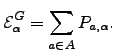
and ![]() . We further define an escape probability for each
. We further define an escape probability for each ![]() as the sum of branching probabilities to nodes in
as the sum of branching probabilities to nodes in ![]() , i.e.
, i.e.
 | (6.12) |
 | (6.13) |
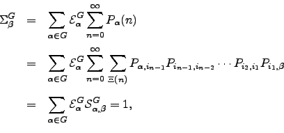
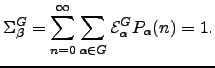
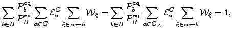
It is clear from the last line of Equation 4.14 that for fixed ![]() the quantities
the quantities ![]() define a probability distribution. However, the pathway sums
define a probability distribution. However, the pathway sums ![]() are not probabilities, and may be greater than unity. In particular,
are not probabilities, and may be greater than unity. In particular, ![]() because the path of zero length is included, which contributes one to the sum. Furthermore, the normalisation condition on the last line of Equation 4.14 places no restriction on
because the path of zero length is included, which contributes one to the sum. Furthermore, the normalisation condition on the last line of Equation 4.14 places no restriction on ![]() terms for which
terms for which ![]() vanishes.
vanishes.
We can also define a probability distribution for individual pathways. Let ![]() be the product of branching probabilities associated with a path
be the product of branching probabilities associated with a path ![]() so that
so that
 | (6.15) |
 | (6.16) |
 | (6.17) |
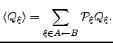
The average of some property, ![]() , defined for each KMC trajectory,
, defined for each KMC trajectory, ![]() , can be calculated from the
, can be calculated from the ![]() as
as
 | (6.18) |
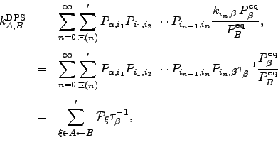
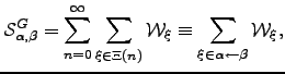
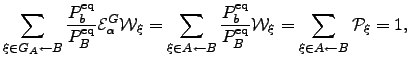
The evaluation of the DPS sum defined in Equation 4.11 can also be rewritten in terms of pathway probabilities:
A digraph representation of the restricted set of pathways defined in Equation 4.19 can be created if we allow sets of sources and sinks to overlap. In that case all the nodes ![]() are defined to be sinks and all the nodes in
are defined to be sinks and all the nodes in ![]() are the sources, i.e. every node in set
are the sources, i.e. every node in set ![]() is both a source and a sink. The required sum then includes all the pathways that finish at sinks of type
is both a source and a sink. The required sum then includes all the pathways that finish at sinks of type ![]() , but not those that finish at sinks of type
, but not those that finish at sinks of type ![]() . The case when sets of sources and sinks (partially) overlap is discussed in detail in Section 4.6.
. The case when sets of sources and sinks (partially) overlap is discussed in detail in Section 4.6.