A general account of the problem of the first passage time in chemical physics was given by Weiss as early as 1965 [212]. In Reference Weiss67 he summarised various techniques for solving such problems to date, and gave a general formula for moments of the first passage time in terms of the Green's function of the Fokker-Plank operator. Explicit expressions for the mean first passage times in terms of the basic transition probabilities for the case of a one-dimensional random walk were obtained by Ledermann and Reuter in 1954 [213], Karlin and MacGregor in 1957 [214], Weiss in 1965 [212], Gardiner in 1985 [215], Van den Broeck in 1988 [216], Le Doussal in 1989 [217], Murthy and Kehr and Matan and Havlin in 1989-1990 [219,211,218], Raykin in 1992 [210], Bar-Haim and Klafter in 1998 [203], Pury and Cáceres in 2003 [220], and Slutsky, Kardar and Mirny in 2004 [221,222]. The one-dimensional random walk is therefore a very well researched topic, both in the field of probability and its physical and chemical applications. The results presented in this section differ in the manner of presentation.
A random walk in a discrete state space ![]() , where all the states can be arranged on a linear chain in such a way that
, where all the states can be arranged on a linear chain in such a way that ![]() for all
for all ![]() , is called a one-dimensional or simple random walk (SRW). The SRW model attracts a lot of attention because of its rich behaviour and mathematical tractability. A well known example of its complexity is the anomalous diffusion law discovered by Sinai [223]. He showed that there is a dramatic slowing down of an ordinary power law diffusion (RMS displacement is proportional to
, is called a one-dimensional or simple random walk (SRW). The SRW model attracts a lot of attention because of its rich behaviour and mathematical tractability. A well known example of its complexity is the anomalous diffusion law discovered by Sinai [223]. He showed that there is a dramatic slowing down of an ordinary power law diffusion (RMS displacement is proportional to ![]() instead of
instead of ![]() ) if a random walker at each site
) if a random walker at each site ![]() experiences a random bias field
experiences a random bias field ![]() . Stanley and Havlin generalised the Sinai model by introducing long-range correlations between the bias fields on each site and showed that the SRW can span a range of diffusive properties [224].
. Stanley and Havlin generalised the Sinai model by introducing long-range correlations between the bias fields on each site and showed that the SRW can span a range of diffusive properties [224].
Although one-dimensional transport is rarely found on the macroscopic scale at a microscopic level there are several examples, such as kinesin motion along microtubules [226,225], or DNA translocation through a nanopore [228,227], so the SRW is interesting not only from a theoretical standpoint. There is a number of models that build upon the SRW that have exciting applications, examples being the SRW walk with branching and annihilation [229], and the SRW in the presence of random trappings [230]. Techniques developed for the SRW were applied to study more complex cases, such as, for example, multistage transport in liquids [231], random walks on fractals [232,233], even-visiting random walks [234], self-avoiding random walks [235], random walks on percolation clusters [237,236], and random walks on simple regular lattices [238,239] and superlattices [240].
A presentation that discusses SRW first-passage probabilities in detail sufficient for our applications is that of Raykin [210]. He considered pathway ensembles explicitly and obtained the generating functions for the occupation probabilities of any lattice site for infinite, half-infinite and finite one-dimensional lattices with the random walker starting from an arbitrary lattice site. As we discuss below, these results have a direct application to the evaluation of the DPS rate constants augmented with recrossings. We have derived equivalent expressions for the first-passage probabilities independently, considering the finite rather than the infinite case, which we discuss in terms of chain digraphs below.
We define a chain as a digraph ![]() with
with ![]() nodes and
nodes and ![]() edges, where
edges, where ![]() and
and ![]() .Adjacent nodes in the numbering scheme are connected via two oppositely directed edges, and these are the only connections. A transition probability
.Adjacent nodes in the numbering scheme are connected via two oppositely directed edges, and these are the only connections. A transition probability ![]() is associated with every edge
is associated with every edge ![]() , as described in Section 4.1.1. An
, as described in Section 4.1.1. An ![]() -node chain is depicted in Figure 4.2 as a subgraph of another graph.
-node chain is depicted in Figure 4.2 as a subgraph of another graph.
![\begin{psfrags}
\psfrag{1} [bc][bc]{$1$}
\psfrag{2} [bc][bc]{$2$}
\psfrag{...
...terline{\includegraphics[width=.52\textheight]{markov/chain.eps}}
\end{psfrags}](img725.png) |
We denote a pathway in ![]() by the ordered sequence of node indices. The length of a pathway is the number of edges traversed. For example, the pathway
by the ordered sequence of node indices. The length of a pathway is the number of edges traversed. For example, the pathway ![]() has length
has length ![]() , starts at node
, starts at node ![]() and finishes at node
and finishes at node ![]() . The indices of the intermediate nodes
. The indices of the intermediate nodes ![]() are given in the order in which they are visited. The product of branching probabilities associated with all edges in a path was defined above as
are given in the order in which they are visited. The product of branching probabilities associated with all edges in a path was defined above as ![]() . For example, the product for the above pathway is
. For example, the product for the above pathway is ![]() , which we can abbreviate as
, which we can abbreviate as ![]() . For a chain graph
. For a chain graph ![]() , which is a subgraph of
, which is a subgraph of ![]() , we also define the set of indices of nodes in
, we also define the set of indices of nodes in ![]() that are adjacent to nodes in
that are adjacent to nodes in ![]() but not members of
but not members of ![]() as
as ![]() . These nodes will be considered as sinks if we are interested in escape from
. These nodes will be considered as sinks if we are interested in escape from ![]() .
.
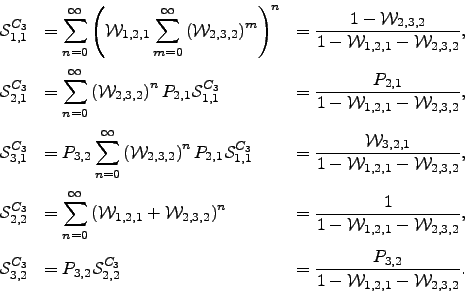
Analytical results for ![]() are easily derived:
are easily derived:
 | (6.25) |
The pathway sums ![]() can be derived for a general chain graph
can be derived for a general chain graph ![]() in terms of recursion relations, as shown in Appendix C. The validity of our results for
in terms of recursion relations, as shown in Appendix C. The validity of our results for ![]() was verified numerically using the matrix multiplication method described in Reference Wales02. For a chain of length
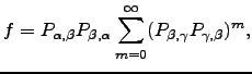
was verified numerically using the matrix multiplication method described in Reference Wales02. For a chain of length ![]() we construct an
we construct an ![]() transition probability matrix
transition probability matrix ![]() with elements
with elements
 | (6.26) |
| (6.27) |
![$\displaystyle \mathcal{S}_{\alpha,\beta}^{C_N} = \sum_{n=1}^{M} \left[ {\bf P}^n \right]_{\alpha,\beta},$](img754.png) | (6.28) |
For chains a sparse-optimised matrix multiplication method for ![]() scales as
scales as ![]() ,and may suffer from convergence and numerical precision problems for larger values of
,and may suffer from convergence and numerical precision problems for larger values of ![]() and branching probabilities that are close to zero or unity [8]. The summation method presented in this section can be implemented to scale as
and branching probabilities that are close to zero or unity [8]. The summation method presented in this section can be implemented to scale as ![]() with constant memory requirements (Algorithm B.1). It therefore constitutes a faster, more robust and more precise alternative to the matrix multiplication method when applied to chain graph topologies (Figure 4.3).
with constant memory requirements (Algorithm B.1). It therefore constitutes a faster, more robust and more precise alternative to the matrix multiplication method when applied to chain graph topologies (Figure 4.3).
![\begin{psfrags}
\psfrag{0.0} [bc][bc]{$0.0$}
\psfrag{0.5} [bc][bc]{$0.5$}
...
...ine{\includegraphics[width=.47\textheight]{markov/alg1VSsmm.eps}}
\end{psfrags}](img758.png) |
Mean escape times for ![]() are readily obtained from the results in Equation 4.24 by applying the method outlined in Section 4.1.5:
are readily obtained from the results in Equation 4.24 by applying the method outlined in Section 4.1.5:
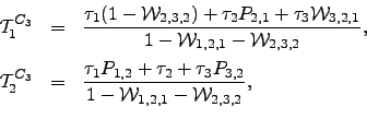 | (6.29) |
The mean escape time from the ![]() graph if started from node
graph if started from node ![]() can be calculated recursively using the results of Appendix D and Section 4.1.5 or by resorting to a first-step analysis [241].
can be calculated recursively using the results of Appendix D and Section 4.1.5 or by resorting to a first-step analysis [241].