


Next: Graph Transformation Method Up: ENSEMBLES OF REARRANGEMENT PATHWAYS Previous: Chain Graphs Contents
Complete Graphs
In a complete digraph each pair of nodes is connected by two oppositely directed edges [155]. The complete graph with  graph nodes is denoted
  , and has nodes and
  edges, remembering that we have two edges per connection (Figure 4.4).
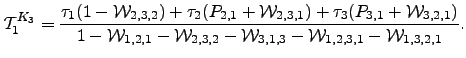
Figure: Complete graphs  and
and  , depicted as the subgraphs of a larger graph. Visible sink nodes are shaded.
 ![\begin{psfrags}
\psfrag{1} [bc][bc]{$1$}
\psfrag{2} [bc][bc]{$2$}
\psfrag{...
...ncludegraphics[width=.52\textheight]{markov/complete_graphs.eps}}
\end{psfrags}](img764.png) |
Due to the complete connectivity we need only consider two cases: when the starting and finishing nodes are the same and when they are distinct. We employ complete graphs for the purposes of generality. An arbitrary graph  is a subgraph of
  with transition probabilities for non-existent edges set to zero. All the results in this section are therefore equally applicable to arbitrary graphs.
 The complete graph will not be considered here as it is topologically identical to the graph  . The difference between the and
  graphs is the existence of edges that connect nodes
  and
and  . Pathways confined to can therefore contain cycles, and for a given path length they are significantly more numerous (Figure 4.5).
Figure: The growth of the number of pathways with the pathway length for and . The starting node is chosen arbitrarily for while for the we start at one of the terminal nodes. Any node adjacent to or is a considered to be a sink and for simplicity we consider only one escape route from every node. Note the log scale on the vertical axis.
 ![\begin{psfrags}
\psfrag{K3} [bc][bc]{$K_3$}
\psfrag{C3} [bc][bc]{$C_3$}
\p...
...ncludegraphics[width=.47\textheight]{markov/number_of_paths.eps}}
\end{psfrags}](img766.png) |
The  can again be derived analytically for this graph:
 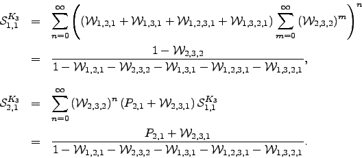 | (6.30) |
The results for any other possibility can be obtained by permuting the node indices appropriately. The pathway sums  for larger complete graphs can be obtained by recursion. For
  any path leaving from and returning to can be broken down into a step out of to any
  , all possible paths between
  and
and  within
  , and finally a step back to from
  . All such paths can be combined together in any order, so we have a multinomial distribution [242]:
 | (6.31) |
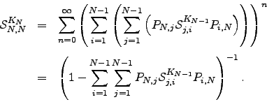
To evaluate  we break down the sum into all paths that depart from and return to , followed by all paths that leave node and reach node 1 without returning to . The first contribution corresponds to a factor of , and the second produces a factor
  for every :
 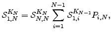 | (6.32) |
where  is defined to be unity. Any other
  can be obtained by a permutation of node labels.
 Algorithm B.2 provides an example implementation of the above formulae optimised for incomplete graphs. The running time of Algorithm B.2 depends strongly on the graph density. (A digraph in which the number of edges is close to the maximum value of is termed a dense digraph [202].) For the algorithm runs in  time, while for an arbitrary graph it scales as
  , where
  is the average degree of the nodes. For chain graphs the algorithm runs in
  time and therefore constitutes a recursive-function-based alternative to Algorithm B.1 with linear memory requirements. For complete graphs an alternative implementation with
  scaling is also possible.
Although the scaling of the above algorithm with may appear disastrous, it does in fact run faster than standard KMC and MM approaches for graphs where the escape probabilities are several orders of magnitude smaller than the transition probabilities (Algorithm B.2). Otherwise, for anything but moderately branched chain graphs, Algorithm B.2 is significantly more expensive. However, the graph-transformation-based method presented in Section 4.4 yields both the pathway sums and the mean escape times for a complete graph in  time, and is the fastest approach that we have found.
Mean escape times for are readily obtained from the results in Equation 4.30 by applying the method outlined in Section 4.1.5:
 | (6.33) |
We have verified this result analytically using first-step analysis and numerically for various values of the parameters  and
and  . and obtained quantitative agreement (see Figure 4.6).
 Figure: Mean escape time from as a function of the escape probability  . The transition probabilities for the graph are parametrised by for simplicity:
 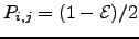 for all
 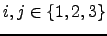 and
and 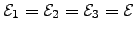 . Kinetic Monte Carlo data (triangles) was obtained by averaging over
  trajectories for each of 33 parameterisations. The solid line is the exact solution obtained using Equation 4.33. The units of
  are arbitrary. Note the log scale on the vertical axis.
 ![\begin{psfrags}
\psfrag{Tau} [bc][bc]{$\log_{10}\mathcal{T}^{K_3}$}
\psfrag{...
...ncludegraphics[width=.47\textheight]{markov/K3_waiting_time.eps}}
\end{psfrags}](img785.png) |
Figure 4.7 demonstrates how the advantage of exact summation over KMC and MM becomes more pronounced as the escape probabilities become smaller. Figure: The computational cost of the kinetic Monte Carlo and matrix multiplication methods as a function of escape probability for (see caption to Figure 4.6 for the definition of ).  is the number of matrix multiplications required to converge the value of the total probability of getting from node to nodes ,
  and : the calculation was terminated when the change in the total probability between iterations was less than
  . The number of matrix multiplications and the average trajectory length
  can be used as a measure of the computational cost of the matrix multiplication and kinetic Monte Carlo approaches, respectively. The computational requirements of the exact summation method are independent of . Note the log scale on the vertical axis.
 ![\begin{psfrags}
\psfrag{M} [bc][bc]{$\log_{10}M$}
\psfrag{n} [bc][bc]{$\log_...
...graphics[width=.47\textheight]{markov/K3_computational_cost.eps}}
\end{psfrags}](img790.png) |
Next: Graph Transformation Method Up: ENSEMBLES OF REARRANGEMENT PATHWAYS Previous: Chain Graphs Contents Semen A Trygubenko 2006-04-10