Here we present a graph transformation (GT) approach for calculating the pathway sums and the mean escape times for ![]() . In general, it is applicable to arbitrary digraphs, but the best performance is achieved when the graph in question is dense. The algorithm discussed in this section will be referred to as DGT (D for dense). A sparse-optimised version of the GT method (SGT) will be discussed in Section 4.5.
. In general, it is applicable to arbitrary digraphs, but the best performance is achieved when the graph in question is dense. The algorithm discussed in this section will be referred to as DGT (D for dense). A sparse-optimised version of the GT method (SGT) will be discussed in Section 4.5.
The GT approach is similar in spirit to the ideas that lie behind the mean value analysis and aggregation/disaggregation techniques commonly used in the performance and reliability evaluation of queueing networks [187,265,267,266]. It is also loosely related to dynamic graph algorithms [270,271,269,268], which are used when a property is calculated on a graph subject to dynamic changes, such as deletions and insertions of nodes and edges. The main idea is to progressively remove nodes from a graph whilst leaving the average properties of interest unchanged. For example, suppose we wish to remove node ![]() from graph
from graph ![]() to obtain a new graph
to obtain a new graph ![]() . Here we assume that
. Here we assume that ![]() is neither source nor sink. Before node
is neither source nor sink. Before node ![]() can be removed the property of interest is averaged over all the pathways that include the edges between nodes
can be removed the property of interest is averaged over all the pathways that include the edges between nodes ![]() and
and ![]() .The averaging is performed separately for every node
.The averaging is performed separately for every node ![]() . Next, we will use the waiting time as an example of such a property and show that the mean first passage time in the original and transformed graphs is the same.
. Next, we will use the waiting time as an example of such a property and show that the mean first passage time in the original and transformed graphs is the same.
The theory is an extension of the results used to perform jumps to second neighbours in previous KMC simulations [272,8]. Consider KMC trajectories that arrive at node ![]() , which is adjacent to
, which is adjacent to ![]() . We wish to step directly from
. We wish to step directly from ![]() to any node in the set of nodes
to any node in the set of nodes ![]() that are adjacent to
that are adjacent to ![]() or
or ![]() , excluding these two nodes themselves. To ensure that the mean first-passage times from sources to sinks calculated in
, excluding these two nodes themselves. To ensure that the mean first-passage times from sources to sinks calculated in ![]() and
and ![]() are the same we must define new branching probabilities,
are the same we must define new branching probabilities, ![]() from
from ![]() to all
to all ![]() , along with a new waiting time for escape from
, along with a new waiting time for escape from ![]() ,
, ![]() . Here,
. Here, ![]() corresponds to the mean waiting time for escape from
corresponds to the mean waiting time for escape from ![]() to any
to any ![]() , while the modified branching probabilities subsume all the possible recrossings involving node
, while the modified branching probabilities subsume all the possible recrossings involving node ![]() that could occur in
that could occur in ![]() before a transition to a node in
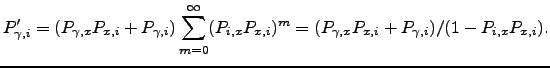
before a transition to a node in ![]() . Hence the new branching probabilities are:
. Hence the new branching probabilities are:
 | (6.34) |
It is easy to show that the new branching probabilities are normalised:
 | (6.35) |
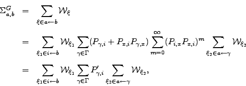
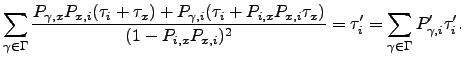
![$\displaystyle \tau_i' = \left[ \frac{d}{d\zeta} \sum_{\gamma\in\Gamma}\frac{P_{...
..._x+\tau_i)}} \right]_{\zeta=0} = \frac{\tau_i+P_{x,i}\tau_x}{1-P_{i,x}P_{x,i}}.$](img801.png) | (6.36) |
 | (6.37) |
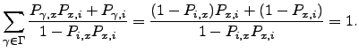
Now consider the effect of removing node ![]() on the mean first-passage time from source
on the mean first-passage time from source ![]() to sink
to sink ![]() ,
, ![]() , using the approach of Section 4.1.4.
, using the approach of Section 4.1.4.
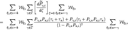
![\begin{displaymath}\begin{array}{lll} \mT _{a,b}^{G'} &=& \displaystyle \left[\f...
...t[ \frac{d\mWt _{\xi_2}}{d\zeta} \right]_{\zeta=0}, \end{array}\end{displaymath}](img807.png) | (6.38) |
 | (6.39) |
 | (6.40) |
 | (6.41) |
The above procedure extends the BKL approach [190] to exclude not only the transitions from the current state into itself but also transitions involving an adjacent node ![]() . Alternatively, this method could be viewed as a coarse-graining of the Markov chain. Such coarse-graining is acceptable if the property of interest is the average of the distribution of times rather than the distribution of times itself. In our simulations the average is the only property of interest. In cases when the distribution itself is sought, the approach described here may still be useful and could be the first step in the analysis of the distribution of escape times, as it yields the exact average of the distribution.
. Alternatively, this method could be viewed as a coarse-graining of the Markov chain. Such coarse-graining is acceptable if the property of interest is the average of the distribution of times rather than the distribution of times itself. In our simulations the average is the only property of interest. In cases when the distribution itself is sought, the approach described here may still be useful and could be the first step in the analysis of the distribution of escape times, as it yields the exact average of the distribution.
The transformation is illustrated in Figure 4.8 for the case of a single source.
![\begin{psfrags}
\psfrag{1} [bc][bc]{$1$}
\psfrag{1'} [bc][bc]{$1'$}
\psfra...
...}
\centerline{\includegraphics{markov/graph_transformation.eps}}
\end{psfrags}](img813.png) |
| |
We now describe algorithms to implement the above approach and calculate mean escape times from complete graphs with multiple sources and sinks. Listings for some of the algorithms discussed here are given in Appendix B. We follow the notation of Section 4.1.4 and consider a digraph ![]() consisting of
consisting of ![]() source nodes,
source nodes, ![]() sink nodes, and
sink nodes, and ![]() intervening nodes.
intervening nodes. ![]() therefore contains the subgraph
therefore contains the subgraph ![]() .
.
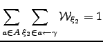
The result of the transformation of a graph with a single source ![]() and
and ![]() sinks using Algorithm B.3 is the mean escape time
sinks using Algorithm B.3 is the mean escape time  and
and ![]() pathway probabilities
pathway probabilities ![]() ,
, ![]() . Solving a problem with
. Solving a problem with ![]() sources is equivalent to solving
sources is equivalent to solving ![]() single source problems. For example, if there are two sources
single source problems. For example, if there are two sources ![]() and
and ![]() we first solve a problem where only node
we first solve a problem where only node ![]() is set to be the source to obtain
is set to be the source to obtain  and the pathway sums from
 ![]() to every sink node
to every sink node ![]() . The same procedure is then followed for
. The same procedure is then followed for ![]() .
.
The form of the transition probability matrix ![]() is illustrated below at three stages: first for the original graph, then at the stage when all the intervening nodes have been removed (line 16 in Algorithm B.3), and finally at the end of the procedure:
is illustrated below at three stages: first for the original graph, then at the stage when all the intervening nodes have been removed (line 16 in Algorithm B.3), and finally at the end of the procedure:
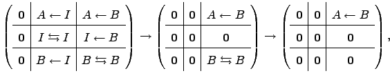 | (6.42) |
Algorithm B.3 uses the adjacency matrix representation of graph ![]() , for which the average of the distribution of mean first passage times is to be obtained. For efficiency, when constructing the transition probability matrix
, for which the average of the distribution of mean first passage times is to be obtained. For efficiency, when constructing the transition probability matrix ![]() we order the nodes with the sink nodes first and the source nodes last. Algorithm B.3 is composed of two parts. The first part (lines 1-16) iteratively removes all the intermediate nodes from graph
we order the nodes with the sink nodes first and the source nodes last. Algorithm B.3 is composed of two parts. The first part (lines 1-16) iteratively removes all the intermediate nodes from graph ![]() to yield a graph that is composed of sink nodes and source nodes only. The second part (lines 17-34) disconnects the source nodes from each other to produce a graph with
to yield a graph that is composed of sink nodes and source nodes only. The second part (lines 17-34) disconnects the source nodes from each other to produce a graph with ![]() nodes and
nodes and ![]() directed edges connecting each source with every sink. Lines 13-15 are not required for obtaining the correct answer, but the final transition probability matrix looks neater.
directed edges connecting each source with every sink. Lines 13-15 are not required for obtaining the correct answer, but the final transition probability matrix looks neater.
The computational complexity of lines 1-16 of Algorithm B.3 is ![]() . The second part of Algorithm B.3 (lines 17-34) scales as
. The second part of Algorithm B.3 (lines 17-34) scales as ![]() . The total complexity for the case of a single source and for the case when there are no intermediate nodes is
. The total complexity for the case of a single source and for the case when there are no intermediate nodes is ![]() and
and ![]() , respectively. The storage requirements of Algorithm B.3 scale as
, respectively. The storage requirements of Algorithm B.3 scale as ![]() .
.
We have implemented the algorithm in Fortran 95 and timed it for complete graphs of different sizes. The results presented in Figure 4.9 confirm the overall cubic scaling. The program is GPL-licensed [273] and available online [274]. These and other benchmarks presented in this chapter were obtained for a single Intel ![]() Pentium
Pentium ![]() 4 3.00GHz 512Kb cache processor running under the Debian GNU/Linux operating system [275]. The code was compiled and optimised using the Intel
4 3.00GHz 512Kb cache processor running under the Debian GNU/Linux operating system [275]. The code was compiled and optimised using the Intel ![]() Fortran compiler for Linux.
Fortran compiler for Linux.
![\begin{psfrags}
\psfrag{CPU time / s} [bc][bc]{CPU time / s}
\psfrag{N} [bc]...
...r][br]{$1000$}
\centerline{\includegraphics{markov/KnCPUofN.ps}}
\end{psfrags}](img831.png) |