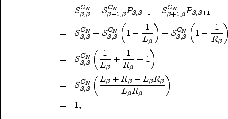
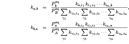
As detailed in Section 4.1.1, within a digraph representation of a coarse-grained PES each minimum is represented by a single node and each transition state is represented by two oppositely directed edges. Here we ignore degenerate rearrangements since they do not affect the rates, and for cases where more than one transition state links the same pair of minima only the one with the fastest forward and backward rates is used. Adopting the non-recrossing DPS rate definition from Equation 4.11 we can associate forward and backward rate constants
 .
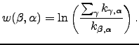
. For a detailed description of Dijkstra and BFM algorithms we refer the reader to Reference CormenLRS01. A suitable choice of edge weight function to be used with either of the shortest path algorithms must be made. We define the weight of each directed edge ![]() as
as
 and
and It makes sense to include only minima with more than one connection when searching for the fastest pathway. In our calculations we first iteratively identified a connected subset of minima with the number of connections greater than one, and then run the above algorithm for this subset.
To find the fastest path connecting minima ![]() and
and ![]() in the direction
in the direction ![]() it is necessary to solve either a single-source shortest paths problem with minimum
it is necessary to solve either a single-source shortest paths problem with minimum ![]() chosen as a source, or a single destination shortest paths problem with minimum
chosen as a source, or a single destination shortest paths problem with minimum ![]() chosen as the destination. In the latter case all the edges in the graph need to be reversed, which can be accomplished by simply swapping the arguments to the weight function in Equation E.2. This reversal is possible because our graph is a symmetric digraph, i.e. if there is an edge
chosen as the destination. In the latter case all the edges in the graph need to be reversed, which can be accomplished by simply swapping the arguments to the weight function in Equation E.2. This reversal is possible because our graph is a symmetric digraph, i.e. if there is an edge ![]() then there is also an edge
then there is also an edge ![]() .
.
A useful check for correct implementation of this algorithm is to verify that the weight of the shortest path from minimum ![]() to minimum
to minimum ![]() ,
, ![]() , is related to the rate
, is related to the rate ![]() calculated for that pathway by
calculated for that pathway by
| (E.3) |
The BFM algorithm runs in 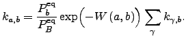 time while Dijkstra's algorithm as described in Reference dijkstra59 scales as
 ![]() [154]. Although both algorithms appear to have similar (quadratic) asymptotic complexity for the case of sparse graphs (e.g.
[154]. Although both algorithms appear to have similar (quadratic) asymptotic complexity for the case of sparse graphs (e.g. ![]() ) the scaling prefactor is smaller for Dijkstra's algorithm. In addition, for sparse graphs with
) the scaling prefactor is smaller for Dijkstra's algorithm. In addition, for sparse graphs with ![]() an implementation of Dijkstra's algorithm that utilises a priority queue of some sort can improve the asymptotic bounds further. Priority queues based on binary min-heap and Fibonacci heap [276] result in
an implementation of Dijkstra's algorithm that utilises a priority queue of some sort can improve the asymptotic bounds further. Priority queues based on binary min-heap and Fibonacci heap [276] result in ![]() and
and ![]() scaling of the algorithm, respectively [154]. In the present work we have used a priority queue based on Fibonacci heap. A performance comparison of our implementations of BFM and static Dijkstra's algorithms is shown in Figure E.1.
scaling of the algorithm, respectively [154]. In the present work we have used a priority queue based on Fibonacci heap. A performance comparison of our implementations of BFM and static Dijkstra's algorithms is shown in Figure E.1.
Since knowledge of all the pathways on a complicated PES is out of the question a representative sample must be obtained to properly describe the property of interest. It is unclear what is the best strategy of evolving the pathway database if the proper description of kinetics is sought, as sampling techniques may introduce a bias towards pathways of particular type.
In previous DPS studies a set of perturbations was applied to the fastest known path to generate new ones [9,10,8]. New pathways were constructed from a subset of stationary points featured in the pathway being perturbed, and from these that were found as a result of perturbation. Because building the shortest paths tree with Dijkstra's algorithm is relatively cheap it is possible to analyse the whole database for the presence of new faster pathways rather than just the subset. Results for an example application are presented in Figure E.2.
![\begin{psfrags}
\psfrag{kABr} [bc][bc]{$\log_{10} k_{a,b}$}
\psfrag{Pathway ...
...cludegraphics[width=.50\textheight]{fastest_path/RateABrofn.eps}}
\end{psfrags}](img987.png) |
Each attempt to shortcut the path was realised as a single connect run (see Chapter 2) seeded with two minima ![]() separated by a gap of length
separated by a gap of length ![]() along the path. If the fastest path
along the path. If the fastest path ![]() found by Dijkstra's algorithm was different (not necessarily new) from the one that was currently being perturbed the iteration was completed, this pathway was perturbed in the next iteration and parameter
found by Dijkstra's algorithm was different (not necessarily new) from the one that was currently being perturbed the iteration was completed, this pathway was perturbed in the next iteration and parameter ![]() was reset to
was reset to ![]() . Otherwise,
. Otherwise, ![]() was incremented by one, unless
was incremented by one, unless ![]() in which case the calculation was terminated.
in which case the calculation was terminated.
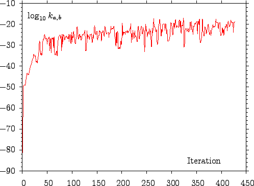 scale on vertical axis. As the generation of new connections can affect the rates of the pathways explicitly recorded in the pathway database (see Equation