Our principal concern in this chapter is the development of the double-ended NEB approach [27–30]. The earliest double-ended methods were probably the linear and quadratic synchronous transit algorithms (LST and QST) [125], which are entirely based on interpolation between the two endpoints. In LST the highest energy structure is located along the straight line that links the two endpoints. QST is similar in spirit, but approximates the reaction path using a parabola instead of a straight line. Neither interpolation is likely to provide a good estimate of the path except for very simple reactions, but they may nevertheless be useful to generate initial guesses for more sophisticated double-ended methods.
Another approach is to reduce the distance between reactant and product by some arbitrary value to generate an ‘intermediate’, and seek the minimum energy of this intermediate structure subject to certain constraints, such as fixed distance to an endpoint. This is the basis of the ‘Saddle’ optimisation method [126] and the ‘Line Then Plane’ [127] algorithm, which differ only in the definition of the subspace in which the intermediate is allowed to move. The latter method optimises the intermediate in the hyperplane perpendicular to the interpolation line, while ‘Saddle’ uses hyperspheres. The minimised intermediate then replaces one of the endpoints and the process is repeated.
There are also a number of methods that are based on a ‘chain-of-states’ (CS) approach, where several images of the system are somehow coupled together to create an approximation to the required path. The CS methods mainly differ in the way in which the initial guess to the path is refined. In the ‘Chain’ method [128] the geometry of the highest energy image is relaxed first using only the component of the gradient perpendicular to the line connecting its two neighbours. The process is then repeated for the next-highest energy neighbours. The optimisation is terminated when the gradient becomes tangential to the path. The ‘Locally Updated Planes’ method [129] is similar, but the images are relaxed in the hyperplane perpendicular to the reaction coordinate, rather than along the line defined by the gradient, and all the images are moved simultaneously.
The NEB approach introduced some further refinements to these CS methods [30]. It is based on a discretised representation of the path originally proposed by Elber and Karplus [88], with modifications to eliminate corner-cutting and sliding-down problems [27], and to improve the stability and convergence properties [29]. Maragakis et al. applied the NEB method to various physical systems ranging from semiconductor materials to biologically relevant molecules. They report that use of powerful minimisation methods in conjunction with the NEB approach was unsuccessful [107]. These problems were attributed to instabilities with respect to the extra parameters introduced by the springs.
The main result of the present contribution is a modified ‘doubly nudged’ elastic band (DNEB) method, which is stable when combined with the L-BFGS minimiser. In comparing the DNEB approach with other methods we have also analysed quenched velocity Verlet minimisation, and determined the best point at which to remove the kinetic energy. Extensive tests show that the DNEB/L-BFGS combination provides a significant performance improvement over previous implementations. We therefore outline a new strategy to connect distant minima, which is based on successive DNEB searches to provide transition state candidates for refinement by eigenvector-following.
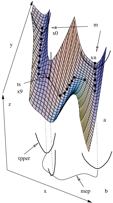
In the present work we used the nudged elastic band [27, 28] (NEB) and eigenvector-following [12–19, 22–24] (EF) methods for locating and refining transition states. In the NEB approach the path is represented as a set of images that connect the endpoints and , where is a vector containing the coordinates of image (Figure 2.1) [29]. In the usual framework of double-ended methodologies [130] the endpoints are stationary points on the PES (usually minima), which are known in advance. In addition to the true potential, , which binds the atoms within each image, equivalent atoms in adjacent images are interconnected by springs according to a parabolic potential,
| (2.1) |
Subsequently these potentials will be referred to as the ‘true potential’ and the ‘spring potential’, respectively.
The springs are intended to hold images on the path during optimisation — otherwise they would slide down to the endpoints, or to other intermediate minima [88]. Occasionally, depending on the quality of the initial guess, we have found that some images may converge to higher index stationary points. One could imagine the whole construction as a band or rope that is stretched across the PES, which, if optimised, is capable of closely following a curve defined in terms of successive minima, transition states, and the intervening steepest-descent paths.
In practice, the above formulation encounters difficulties connected with the coupling between the ‘true’ and ‘spring’ components of the potential. The magnitude of the springs’ interference with the true potential is system dependent and generally gives rise to corner-cutting and sliding-down problems [27]. It is convenient to discuss these difficulties in terms of the components of the true gradient, , and spring gradient, , parallel and perpendicular to the path. The parallel component of the gradient at image on the path is obtained by projecting out the perpendicular component using an estimate of the tangent to the path. The parallel and perpendicular components for image are:
| (2.2) |
where , the unit vector is the tangent, and denotes the scalar product of vectors and . Here and throughout this work we denote unit vectors by a hat. The complete gradient, , has components for a band of images with atomic degrees of freedom each.
Corner-cutting has a significant effect when a path experiences high curvature. Here is large, which prevents the images from following the path closely because the spring force necessarily has a significant component perpendicular to the tangent. The sliding-down problem occurs due to the presence of , which perturbs the distribution of images along the path, creating high-resolution regions (around the local minima) and low-resolution regions (near the transition states) [27]. Both problems significantly affect the ability of the NEB method to produce good transition state candidates. We have found that sliding-down and corner-cutting are interdependent and cannot both be remedied by adjusting the spring force constant ; increasing may prevent sliding-down but it will make corner-cutting worse.
The aforementioned problems can sometimes be eliminated by constructing the NEB gradient from the potential in the following way: and are projected out, which gives the elastic band its ‘nudged’ property [28]. Removal of can be thought of as bringing the path into a plane or flattening the PES [Figure 2.1 (b)], while removal of is analogous to making the images heavier so that they favour the bottom of the valley at all times.
The choice of a method to estimate the tangent to the path is important for it affects the convergence of the NEB calculation. Originally, the tangent vector, , for image was obtained by normalising the line segment between the two adjacent images, and [27]:
| (2.3) |
However, kinks can develop during optimisation of the image chain using this definition of . It has been shown [29] that kinks are likely to appear in the regions where the ratio is larger than the length of the line segment, , used in estimating the tangent [Figure 2.2 (a)].
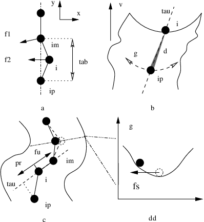
Both the above ratio, the image density and can vary depending on the system of interest, the particular pathway and other parameters of the NEB calculation. From Equation 2.3 it can be seen that , and, hence, the next step in the optimisation of image , is determined by its neighbours, which are not necessarily closer to the path than image . Therefore, a better approach in estimating the would be to use only one neighbour, since then we only need this neighbour to be better converged than image .
There are two neighbours to select from, and it is natural to use the higher-energy one for this purpose, since steepest-descent paths are easier to follow downhill than uphill:
| (2.4) |
where and are two adjacent images with energies and , and . In this way, an image that has one higher-energy neighbour behaves as if it is ‘hanging’ on to it [Figure 2.2(b)].
The above tangent formulation requires special handling of extrema along the path, and a mechanism for switching at such points was proposed [29]. It also fails to produce an even distribution of images in regions with high curvature [Figure 2.2 (c)]. We presume that Henkelman and Jónsson substitute by in Equation 2.2 to obtain a spring gradient formulation that will keep the images equispaced when the tangent from Equation 2.4 is used in the projections [28]:
| (2.5) |
In the present work the NEB approach has been used in combination with two minimisers, namely the quenched velocity Verlet (QVV) and the limited-memory Broyden-Fletcher-Goldfarb-Shanno (L-BFGS) algorithms. It is noteworthy that the objective function corresponding to the projected NEB gradient is unknown, but it is not actually required in either of the minimisation algorithms that we consider.
Optimisation is a general term that refers to finding stationary points of a function. Many problems in computational chemistry can be formulated as optimisation of a multidimensional function, NEB optimisation being one of the many. The goal of an optimisation problem can be formulated as follows: find a combination of parameters (independent variables) that optimise a given quantity (the objective function), possibly with some restrictions on the allowed parameter ranges [131]. To know exactly what we are looking for optimality conditions need to be defined. The condition
| (2.6) |
where is the set of all possible values of the control variable , defines the global optimum of the function . For an unconstrained problem is infinitely large, and finding the corresponding global minimum may be a difficult task. Similarly, a point is a strong local minimum of if
| (2.7) |
where is a set of feasible points contained in the neighbourhood of . For a weak local minimum only an inequality must be satisfied in Equation 2.7.
More easily identified optimality conditions could be used instead of Equation 2.6 and Equation 2.7 if is a function with continuous first and second derivatives, namely, the stationary point and the strong local minimum conditions. A stationary point is a point where the gradient vanishes:
| (2.8) |
and a strong local minimum is a stationary point where the Hessian matrix
| (2.9) |
is positive-definite:
| (2.10) |
Formally, optimisation of an NEB qualifies as a nonlinear unconstrained continuous multivariable optimisation problem. There are many algorithms available for solving problems of this type that differ in their computational requirements, convergence and other properties. However, NEB optimisation is augmented with an additional difficulty: due to the projections involved the objective function that is being minimised is unknown. Nevertheless, several optimisation techniques were found to be stable in working with NEB. Most of these are based on steepest-descent methods and, consequently, are not very efficient. The L-BFGS and QVV minimisers discussed in this section are based on the deterministic approach for finding local minima.
The basic structure of any local minimiser can be summarised as follows:
The descent direction is defined as the one along which the directional derivative is negative:
| (2.11) |
Negativity of the left hand side guarantees that a lower function value will be found along provided that the step is sufficiently small. According to the way algorithms choose the search direction they are classified as non-derivative, gradient and second-derivative. Steepest-descent is an example of a gradient-based method, while BFGS belongs to the class of quasi-Newton methods (or quasi-second-derivative methods). The steepest-descent search direction is defined as the direction antiparallel to the gradient at the current point
| (2.12) |
whereas second-derivative-based methods determine the search direction using the Newton-Raphson equation [31]:
| (2.13) |
The step length can be determined using either ‘line search’ or ‘trust radius’ approaches. Line search is essentially a one-dimensional minimisation of the function , which is performed at every step [131]. In the trust-radius-based approach the step length is adjusted dynamically depending on how well the minimisation algorithm predicts the change in the object function value [9]. There is no clear evidence for the superiority of one method over the other [131]; however, in combination with the limited-memory version of BFGS algorithm the trust ratio approach was found to be more efficient for treating problems with discontinuities such as problems involving periodic boundary conditions with cutoffs [9].
The QVV method is based on the velocity Verlet algorithm [32] (VV) as modified by Jónsson et al. [27], and was originally used for NEB optimisation. VV is a symplectic integrator that enjoys widespread popularity, primarily in molecular dynamics (MD) simulations where it is used for numerical integration of Newton’s equations of motion. Its main advantage over the standard Verlet method is the minimisation of the round-off errors. At each time step the coordinates and the velocities are updated from the coupled first-order differential equations in the following manner [32]:
where is the atomic mass. The algorithm involves two stages, with a force evaluation in between. First the positions are updated according to Equation 2.14, and the velocities at midstep are then computed using Equation 2.15. After the evaluation of the gradient at time the velocity is updated again [Equation 2.16] to complete the move. To obtain minimisation it is necessary to remove kinetic energy, and this can be done in several ways. If the kinetic energy is removed completely every step the algorithm is equivalent to a steepest-descent minimisation, which is rather inefficient. Instead, it was proposed by Jónsson et al. [27] to keep only the velocity component that is antiparallel to the gradient at the current step. If the force is consistently pointing in the same direction the system accelerates, which is equivalent to increasing the time step [27]. However, a straightforward variable time step version of the above algorithm was reported to be unsuccessful [110].
The BFGS algorithm belongs to the class of variable metric methods and is slightly different from the Davidon-Fletcher-Powell (DFP) method in the way in which the correction term is constructed [132] (see below). It has become generally recognised that the BFGS algorithm is superior to DFP in convergence tolerances, roundoff error and other empirical issues [31]. The idea of the variable metric, or quasi-Newton, method is to build up a good approximation to the inverse Hessian matrix by constructing a sequence of matrices with the following property:
| (2.17) |
If we are successful in doing so, combining two Newton-Raphson equations (see Equation 2.13) for consecutive iterations and , we find that should satisfy
| (2.18) |
where we have used the property , which must hold if both and are in the neighbourhood of minimum .
At every iteration the new approximation to the inverse Hessian should be constructed in order to calculate the next step. The update formula must be consistent with Equation 2.18 and could take the form
| (2.19) |
where the correction term is constructed using the gradient difference , the step , and the inverse Hessian matrix from the previous iteration . The BFGS update correction is [31]
| (2.20) |
where denotes the direct product of two vectors, and .
Since at every iteration the old Hessian is overwritten with a new one storage locations are needed. This is an entirely trivial disadvantage over the conjugate gradient methods for any modest value of [31]. However, for large-scale problems it is advantageous to be able to specify the amount of storage BFGS is allowed to use.
There is a version of the BFGS algorithm that allows us to vary the amount of storage available to BFGS and is particularly suitable for large-scale problems [2]. The difference between this limited memory BFGS (L-BFGS) algorithm and the standard BFGS is in the Hessian matrix update. L-BFGS stores each correction separately and the Hessian matrix is never formed explicitly. To store each correction to the Hessian storage locations are needed [1]. The user can specify the number of corrections L-BFGS is allowed to store. Every iteration is computed according to a recursive formula described by Nocedal [1]. For the first iterations L-BFGS is identical to the BFGS method. After the first iterations the oldest correction is discarded. Thus, by varying the iteration cost can also be controlled, which makes the method very efficient and flexible. In general, because only recent corrections are stored L-BFGS is better able to use additional storage to accelerate convergence. Here we employed a modified version of Nocedal’s L-BFGS implementation [3] in which the line search was removed and the maximum step size was limited for each image separately.
Single-ended methods use only the function and its derivatives to search for a transition state from the starting point (the initial guess). Since a transition state is a local maximum in one direction but a minimum in all the others it is not generally possible to use standard minimisation methods for this purpose.
Newton-type optimisation methods are based on approximating the objective function locally by a quadratic model and then minimising that function approximately using, for example, the Newton-Raphson (NR) approach [31]. However, the NR algorithm can converge to a stationary point of any index [130]. To converge to a transition state the algorithm may need to start from a geometry at which the Hessian has exactly one negative eigenvalue and the corresponding eigenvector is at least roughly parallel to the reaction coordinate. Locating such a point can be a difficult task and several methods have been developed that help to increase the basins of attraction of transition states, which gives more freedom in choosing the starting geometry [9, 19, 22, 24].
The most widely used single-ended transition state search method is eigenvector-following (EF). In it simplest form it requires diagonalisation of the Hessian matrix [12–15]. For larger systems it is advantageous to use hybrid EF methods that avoid either calculating the Hessian or diagonalising it [8, 22, 23, 133].
We start by reviewing the theory behind the Newton-Raphson methods. Solving the eigenvalue problem
| (2.21) |
yields the matrix , the columns of which are the eigenvectors , and the diagonal matrix , with eigenvalues on the diagonal. The matrix defines a unitary transformation to a new orthogonal basis , in which the original Hessian matrix is diagonal
| (2.22) |
so that Equation 2.13 is simplified to
| (2.23) |
where is the gradient vector in the new basis, which is related to the original gradient vector as
| (2.24) |
because of the unitarity of
| (2.25) |
The unnormalised search direction is defined similarly.
After taking a step of length in the direction , as prescribed by Equation 2.23, the energy changes by
| (2.26) |
provided our quadratic approximation to is perfect. In general and terms in Equation 2.26 with and increase and decrease the energy, respectively. For isolated molecules and bulk models with periodic boundary conditions the Hessian matrix is singular: there are three zero eigenvalues that correspond to overall translations. Non-linear isolated molecules have three additional zero eigenvalues due to rotations. Luckily, in all cases for which the analytic form of the corresponding eigenvectors is known so the eigenvalue shifting procedure could be applied:
| (2.27) |
where are the new eigenvalues. In this work all the zero eigenvalues were shifted by the same amount (). As a result, and problems with applying Equation 2.23 do not arise.
The analytic forms of the ’s corresponding to translations along the , and directions are
| (2.28) |
respectively. The eigenvector that corresponds to rotation about the axis by a small angle can be obtained as
| (2.29) |
where is a normalised -dimensional vector describing the position before the rotation, and is Maclaurin series expansion of the -dimensional rotation matrix [134] with respect to a small angle truncated to the second order. The displacement vectors due to infinitesimal rotation about the , and axes are therefore
| (2.30) |
respectively.
If started from a point at which the Hessian matrix has negative eigenvalues, the NR method is expected to converge to a stationary point of index . However, the step taking procedure may change the index as optimisation proceeds.
Introducing Lagrange multipliers allows a stationary point of specified index to be located. Consider a Lagrangian function
| (2.31) |
where a separate Lagrange multiplier is used for every eigendirection , is a constraint on the step , is the th eigenvalue of , which is defined in Equation 2.27, and is the point about which the potential energy function was expanded. Primes, as before, denote that components are expressed in the orthogonal basis. Differentiating Equation 2.31 with respect to and using the condition for a stationary point the optimal step can be obtained:
| (2.32) |
The predicted energy change corresponding to this step is
| (2.33) |
We have some freedom in choosing the Lagrange multipliers as long as for the eigendirections for which an uphill (downhill) step is to be taken (). The following choice of Lagrange multipliers allows the recovery of the Newton-Raphson step in the vicinity of a stationary point [9]:
| (2.34) |
with the plus sign for an uphill step, and the minus sign for a downhill step.
In cases when Hessian diagonalisation is impossible or undesirable the smallest eigenvalue and a corresponding eigenvector can be found using an iterative method [135].
The springs should distribute the images evenly along the NEB path during the optimisation, and the choice of must be made at the beginning of each run. It has been suggested by Jónsson and coworkers that since the action of the springs is only felt along the path the value of the spring constant is not critical as long as it is not zero [27]. If is set to zero then sensible behaviour occurs for the first several tens of iterations only; even though is projected out, fluctuates and further optimisation will eventually result in the majority of images gradually sliding down to local minima [27].
In practice we find that the value of affects the convergence properties and the stability of the optimisation process. This result depends on the type of minimiser employed and may also depend on minimiser-specific settings. Here we analyse the convergence properties of NEB minimisations using the QVV minimiser (NEB/QVV) and their dependence on the type of velocity quenching. From previous work it is not clear when is the best time to perform quenching during the MD minimisation of the NEB [27–29]. Since the VV algorithm calculates velocities based on the gradients at both current and previous steps quenching could be applied using either of these gradients.
Specifically, it is possible to quench velocities right after advancing the system using Equation 2.14, at the half-step in the velocity evaluation (quenching intermediate velocities at time ) using either the old or new gradient [Equation 2.15], or after completion of the velocity update. In Figure 2.4 we present results for the stability of NEB/QVV as a function of the force constant parameter for three of these quenching approaches. We will refer to an NEB optimisation as stable for a certain combination of parameters (e.g. time integration step, number of images) if the NEB steadily converges to a well-defined path and/or stays in its proximity until the maximal number of iterations is reached or the convergence criterion is satisfied.
We have performed some of the tests on the Müller-Brown (MB) two-dimensional surface [25]. This widely used surface does not present a very challenging or realistic test case, but if an algorithm does not behave well for this system it is unlikely to be useful. MB potential is defined as a sum of four terms, each of which takes the form
| (2.35) |
where and are variables and , , , , and are parameters. In the form these parameters can be written down as , , and . A contour plot of Müller-Brown surface is depicted in Figure 2.3. 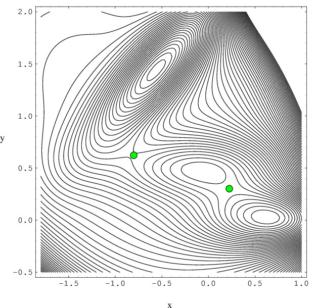
Figure 2.4 shows the results of several thousand optimisations for a 17-image band with the MB two-dimensional potential [25] using QVV minimisation and a time step of (consistent units) for different values of . 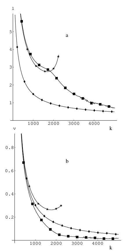
Each run was started from the initial guess obtained using linear interpolation and terminated when the root-mean-square (RMS) gradient became less than . We define the RMS gradient for the NEB as
| (2.36) |
where is the number of images in the band and is the number of atomic degrees of freedom available to each image.
It seems natural to remove the velocity component perpendicular to the gradient at the current point when the geometry , gradient and velocity are available, i.e.
| (2.37) |
where is the velocity vector after quenching. However, we found this approach to be the least stable of all — the optimisation was slow and convergence was very sensitive to the magnitude of the time step. Hence we do not show any results for this type of quenching.
From Figure 2.4 (a) we see that the best approach is to quench the velocity after the coordinate update. The optimisation is then stable for a wide range of force constant values, and the images on the resulting pathway are evenly distributed. In this quenching formulation the velocity response to a new gradient direction is retarded by one step in coordinate space: the step is still taken in the direction but the corresponding velocity component is removed. To implement this slow-response QVV (SQVV) it is necessary to modify the VV algorithm described in Section 2.5.1 by inserting Equation 2.37 in between the two stages described by Equation 2.14 and Equation 2.15.
The second-best approach after SQVV is to quench the velocity at midstep using the new gradient. On average, this algorithm takes twice as long to converge the NEB to a given RMS gradient tolerance compared to SQVV. However, the method is stable for the same range of spring force constant values and produces a pathway in which the images are equispaced more accurately than the other formulations [see Figure 2.4 (b)].
The least successful of the three QVV schemes considered involves quenching velocities at mid-step using the gradient from the previous iteration (stars in Figure 2.4). Even though the number of iterations required is roughly comparable to that obtained by quenching using the new gradient, it has the smallest range of values for the force constant where it is stable. Some current implementations of NEB [136, 137] (intended for use in combination with electronic structure codes) use this type of quenching in their QVV implementation.
We have also conducted analogous calculations for more complicated systems such as permutational rearrangements of Lennard-Jones clusters. The results are omitted for brevity, but agree with the conclusions drawn from the simpler 2D model described above. The same is true for the choice of force constant investigated in the following section.
We find that if the force constant is too small many more iterations are needed to converge the images to the required RMS tolerance, regardless of the type of quenching. In addition, the path exhibits a more uneven image distribution. This result occurs because at the initial stage the images may have very different gradients from the true potential along the band, because they lie far from the required path, and the gradient of the true potential governs the optimisation. When the true RMS force is reduced the springs start to play a more important role. But at this stage the forces are small and so is the QVV step size. The influence of the springs is actually most important during the initial optimisation stage, for it can determine the placement of images in appropriate regions. It is less computationally expensive to guide an image into the right region at the beginning of an optimisation than to restore the distribution afterwards by dragging it between two minima through a transition state region.
If is too big the NEB never converges to the required RMS gradient tolerance value. Instead, it stays in proximity to the path but develops oscillations: adjacent images start to move in opposite directions. For all types of quenching we observed similar behaviour when large values of the force constant were used. This problem is related to the step in coordinate space that the optimiser is taking: for the SQVV case simply decreasing the time step remedies this problem.
We tested the NEB/L-BFGS method by minimising a 17-image NEB for the two-dimensional Müller-Brown surface [25]. Our calculations were carried out using the OPTIM program [138]. The NEB method in its previous formulation [28] and a modified L-BFGS minimiser [9] were implemented in OPTIM in a previous discrete path sampling study [8]. We used the same number of images, initial guess and termination criteria as described in Section 2.5.1 to make the results directly comparable.
Figure 2.5 shows the performance of the L-BFGS minimiser as a function of . We used the following additional L-BFGS specific settings. The number of corrections in the BFGS update was set to (Nocedal’s recommendation for the number of corrections is , see Reference [3]), the maximum step size was , and we limited the step size for each image separately, i.e.
| (2.38) |
where is the step for image . The diagonal elements of the inverse Hessian were initially set to .
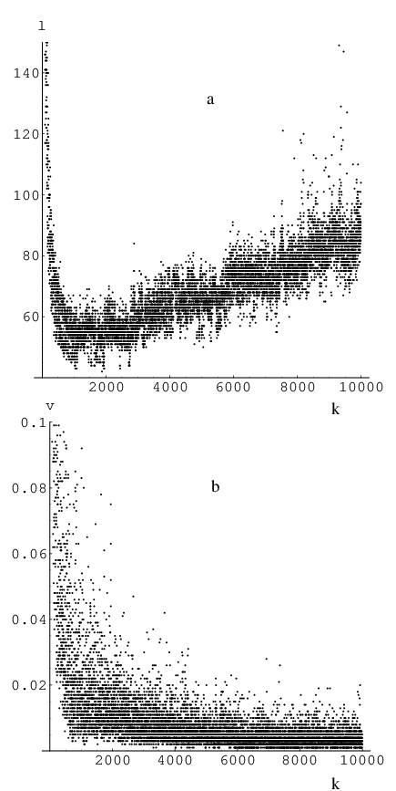
From Figure 2.5 it can be seen that the performance of L-BFGS minimisation is relatively independent of the choice of force constant. All the optimisations with converged to the steepest-descent path, and, for most of this range, in less than 100 iterations. This method therefore gives roughly an order of magnitude improvement in speed over SQVV minimisation [see Figure 2.4 (a)].
We found it helpful to limit the step size while optimising the NEB with the L-BFGS minimiser. The magnitude and direction of the gradient on adjacent images can vary significantly. Taking bigger steps can cause the appearance of temporary discontinuities and kinks in the NEB. The NEB still converges to the correct path, but it takes a while for these features to disappear and the algorithm does not converge any faster.
The NEB/QVV approach has previously been systematically tested on systems with around degrees of freedom [107]. However, in the majority of cases these test systems could be divided into a ‘core’ and a smaller part that actually changes significantly. The number of active degrees of freedom is therefore significantly smaller than the total number in these tests. For example, prototropic tautomerisation of cytosine nucleic acid base () involves motion of one hydrogen atom along a quasi-rectilinear trajectory accompanied by a much smaller distortion of the core.
We have therefore tested the performance of the NEB/SQVV and NEB/L-BFGS schemes for more complicated rearrangements of Lennard-Jones (LJ) clusters to validate the results of Section 2.5.2, and to investigate the stability and performance of both approaches when there are more active degrees of freedom. Most of our test cases involve permutational isomerisation of the LJ, LJ and LJ clusters. These examples include cases with widely varying separation between the endpoints, integrated path length, number of active degrees of freedom and cooperativity.
Permutational rearrangements are particularly interesting because it is relatively difficult to produce an initial guess for the NEB run. In contrast, linear interpolation between the endpoints was found to provide a useful initial guess for a number of simpler cases [27]. For example, it was successfully used to construct the NEB for rearrangements that involve one or two atoms following approximately rectilinear trajectories, and for migration of a single atom on a surface [107]. For more complex processes an alternative approach adopted in previous work is simply to supply a better initial guess ‘by hand’, e.g. construct it from the images with unrelaxed geometries containing no atom overlaps [107]. The ‘detour’ algorithm described in previous calculations that employ the ridge method could also be used to avoid ‘atom-crashing’ in the initial interpolation [93].
It has previously been suggested that it is important to eliminate overall rotation and translation (ORT) of each image during the optimisation of an NEB [27]. We have implemented this constraint in the same way as Jónsson et al., by freezing one atom, restricting the motion of a second atom to a plane, and constraining the motion of a third atom to a line by zeroing the appropriate components of the NEB gradient.
We were able to obtain stable convergence in NEB/L-BFGS calculations only for simple rearrangements, which confirms that straightforward L-BFGS optimisation of the NEB is unstable [107]. Figure 2.6 shows the performance of the NEB/SQVV [Figure 2.6 (a)] and NEB/L-BFGS [Figure 2.6 (b)] approaches for one such rearrangement. These calculations were carried out using a 7-image NEB both with (diamonds) and without (stars) removing ORT for isomerisation of an LJ cluster (global minimum second-lowest minimum). The number of iterations, , is proportional to the number of gradient evaluations regardless of the type of minimiser. Hence, from Figure 2.6 we conclude that for this system NEB/L-BFGS is faster than NEB/SQVV by approximately two orders of magnitude. However, removal of ORT leads to instability in the NEB/L-BFGS optimisation: the images do not stay in proximity to the required path for long and instead diverge from it [see inset in Figure 2.6 (b)].
By experimentation we have found that the main source of the instabilities is the complete removal of . Instead, the inclusion of some portion of in the NEB gradient, i.e.
| (2.39) |
where , makes the NEB/L-BFGS calculations stable but introduces some additional corner-cutting, as well as an extra parameter, . Since we use the transition state candidates from NEB as starting points for further EF calculations the corner-cutting is not a drawback as long as the transition state candidates are good enough. By adjusting in the range of we were able to achieve satisfactory performance for the NEB/L-BFGS method in a number of cases. However, an alternative modification, described below, proved to be even more successful.
The drawback of the NEB gradient described by Equation 2.39 stems from the interference of and , and becomes particularly noticeable when the projection of on and itself are of comparable magnitude. This problem is analogous to the interference of and in the original elastic band method, which was previously solved by ‘nudging’ [28]. We have therefore constructed the gradient of a new ‘doubly’ nudged elastic band (DNEB) using
| (2.40) |
In this formulation some corner-cutting may still occur because the images tend to move cooperatively during optimisation; the spring gradient acting on one image can still indirectly interfere with the true gradients of its neighbours. In our calculations this drawback was not an issue, since we are not interested in estimating properties of the path directly from its discrete representation. Instead we construct it from steepest-descent paths calculated after converging the transition states tightly using the EF approach. We have found DNEB perfectly adequate for this purpose.
We have implemented DNEB method in our OPTIM program [138]. Equation 2.2 was used to obtain components of both spring gradient and true gradient, Equation 2.4 to calculate pathway tangent, and Equations 2.39-2.40 to evaluate the final DNEB gradient. We note that although we employed the improved tangent from Equation 2.4, we did not use Equation 2.5 to obtain . This implementation detail was not clarified in Reference [7], and we thank Dr. Dominic R. Alfonso for pointing that out.
We have also tested a number of approaches that might be useful if one wants to produce a full pathway involving a number of transition states for a complicated rearrangement in just one NEB run. One of these, for instance, is a gradual removal of the component from the NEB gradient once some convergence criterion is achieved. This removal works remarkably well, particularly in situations with high energy initial guesses, which occur frequently if the guessing is fully automated. This adjustment can be thought of as making the band less elastic in the beginning in order to resolve the highest-energy transition state regions first.
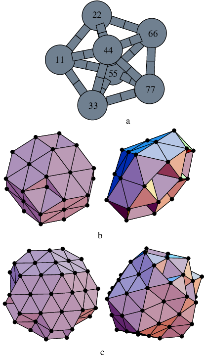
It is sometimes hard to make a direct comparison of different double-ended methods for a particular rearrangement because the calculations may converge to different paths. Another problem concerns the choice of a consistent termination criterion: the RMS force usually converges to some finite system-dependent value, which in turn may depend on the number of images and other parameters. A low-energy chain of NEB images does not necessarily mean that a good pathway has been obtained, since it may arise because more images are associated with regions around local minima, rather than the higher energy transition state regions. Here we present the results of DNEB/L-BFGS, DNEB/SQVV and, where possible, NEB/SQVV calculations for all the distinct permutational rearrangements of the global minimum for the LJ cluster (see Figure 2.7 for the endpoints and nomenclature).
It is possible to draw a firm conclusion as to how well the NEB represents the pathway when the corresponding stationary points and steepest-descent paths are already known. We therefore base our criterion for the effectiveness of an NEB calculation on whether we obtain good estimates of all the transition states. By considering several systems of increasing complexity we hope to obtain comparisons that are not specific to a particular pathway.
Connections between two minima are defined by calculating an approximation to the two steepest-descent paths that lead downhill from each transition state, and two transition states are considered connected if they are linked to the same minimum via a steepest-descent path. We will say that minima are ‘connected’ if there exists a path consisting of one or more transition states and intermediate minima linking them. Permutational isomers of the same minimum are distinguished in these calculations. We refer to the chain of images produced by the NEB calculation as ‘connected’ if going downhill from each transition state using steepest-descent minimisation yields a set of minima that contains the endpoints linked together.
For NEB/SQVV calculations we used the NEB formulation defined in Reference [28]. DNEB is different from the above method because it includes an additional component in the NEB gradient, as described by Equation 2.39 and Equation 2.40. In addition, for the following DNEB calculations we did not remove overall rotation and translation (ORT), because we believe it is unnecessary when our gradient modification is used. To converge transition state candidates tightly we employed EF optimisation, limiting the maximum number of EF iterations to five with an RMS force convergence tolerance of . (Standard reduced units for the Lennard-Jones potential are used throughout this work.) Initial guesses for all the following calculations were obtained by linear interpolation between the endpoints. To prevent ‘atom-crashing’ from causing overflow in the initial guess we simply perturbed such images slightly using random atomic displacements of order reduced units.
In each case we first minimised the Euclidean distance between the endpoints with respect to overall rotation and translation using the method described in Reference [142].∗ SQVV minimisation was performed with a time step of and a maximum step size per degree of freedom of . This limit on the step size prevents the band from becoming ‘discontinuous’ initially and plays an important role only during the first or so iterations. The limit was necessary because for the cases when the endpoints are permutational isomers linear interpolation usually yields bands with large gradients, and it is better to refrain from taking excessive steps at this stage. We did not try to select low energy initial guesses for each rearrangement individually, since one of our primary concerns was to automate this process. For the same reason, all the L-BFGS optimisations were started from guesses preoptimised using SQVV until the RMS force dropped below .
Table 2.1 shows the minimum number of images and gradient calls required to produce a connected pathway using the DNEB/L-BFGS and DNEB/SQVV methods. These calculations were run assuming no prior knowledge of the path. Normally there is no initial information available on the integrated path length or the number of intermediate minima between the endpoints, and it takes some experimentation to select an appropriate number of images. Our strategy is therefore to gradually increase the number of images to make the problem as computationally inexpensive as possible. Hence we increment the number of images and maximum number of NEB iterations in each calculation until a connected path is produced, in the sense defined above. The permitted image range was and the maximum number of NEB iterations ranged from . We were unable to obtain connected pathways for any of the four LJ rearrangements using the NEB/SQVV approach.
Method 1–2 2–3 3–4 4–5 DNEB/L-BFGS 5(1720) 18(30276) 11(2486) 18(8010) DNEB/SQVV 16(21648) – 10(14310) –
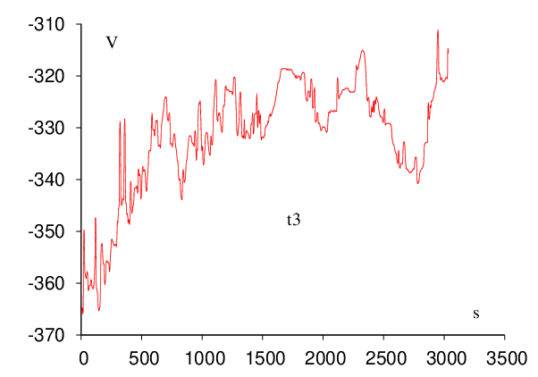
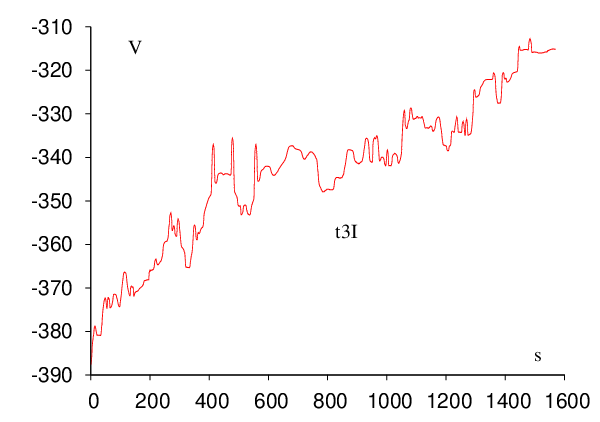
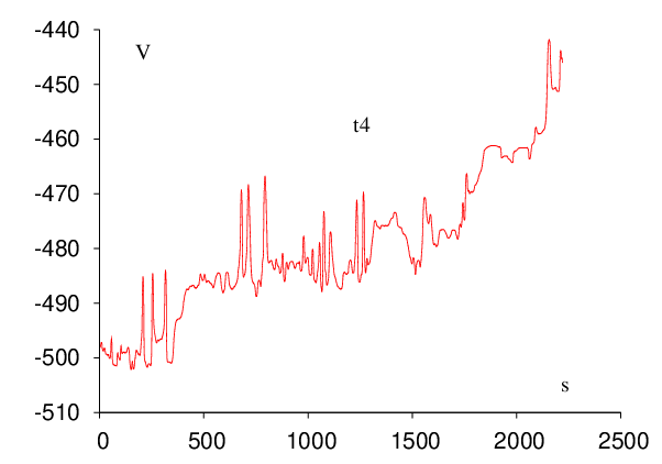
Table 2.2 presents the results of analogous calculations where we keep the number of images fixed to 50. Unlike the performance comparison where the number of images is kept to a minimum (Table 2.1), these results should provide insight into the performance of the DNEB approach when there are sufficient images to resolve all the transition states. All the optimisations for a particular rearrangement converged to the same or an enantiomeric pathway unless stated otherwise. The energy profiles that correspond to these rearrangements are shown in Figure 2.8.
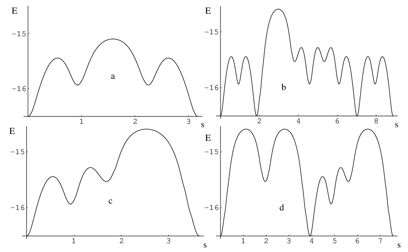
The number of iterations is the sum of the SQVV preoptimisation steps (100 on average) and the actual number of iterations needed by L-BFGS minimiser. This value is not directly comparable since DNEB converged to a different path that contains more intermediate minima. Dashes signify cases where we were unable to obtain a connected pathway. Method 1–2 2–3 3–4 4–5 DNEB/L-BFGS 131 493 171 326 DNEB/SQVV 1130 15178 2777 23405 NEB/SQVV 11088 – 30627 –
From Table 2.1 and Table 2.2 we conclude that in all cases the DNEB/L-BFGS approach is more than an order of magnitude faster than DNEB/SQVV. It is also noteworthy that the DNEB/SQVV approach is faster than NEB/SQVV because overall rotation and translation are not removed. Allowing the images to rotate or translate freely can lead to numerical problems, namely a vanishing norm for the tangent vector, when the image density is very large or the spring force constant is too small. However, when overall rotation and translation are not allowed there is less scope for improving a bad initial guess, because the images are more constrained. This constraint usually means that more images are needed or a better initial guess is required. Our experience is that such constraints usually slow down convergence, depending on which degrees of freedom are frozen: if these are active degrees of freedom (see above) the whole cluster must move instead, which is usually a slow, concerted multi-step process.
In previous work we have used the NEB approach to supply transition state guesses for further EF refinement [8, 133]. Double-ended searches are needed in these discrete path sampling runs to produce alternative minimum–transition state–minimum sequences from an initial path. The end minima that must be linked in such calculations may be separated by relatively large distances, and a detailed algorithm was described for building up a connected path using successive transition state searches. The performance of the DNEB/L-BFGS approach is sufficiently good that we have changed this connection strategy in our OPTIM program. In particular, the DNEB/L-BFGS method can often provide good candidates for more than one transition state at a time, and may even produce all the necessary transition states on a long path. However, it is still generally necessary to consider multiple searches between different minima in order to connect a pair of endpoints. In particular, we would like to use the minimum number of NEB images possible for reasons of efficiency, but automate the procedure so that it eventually succeeds or gives up after an appropriate effort for any pair of minima that may arise in a discrete path sampling run. These calculations may involve the construction of many thousands of discrete paths. As in previous work we converge the NEB transition state candidates using eigenvector-following techniques and then use L-BFGS energy minimisation to calculate approximate steepest-descent paths. These paths usually lead to local minima, which we also converge tightly. The combination of NEB and hybrid eigenvector-following techniques [22, 23] is similar to using NEB with a ‘climbing image’ as described in Reference [29].
The initial parameters assigned to each DNEB run are the number of images and the number of iterations, which we specify by image and iteration densities. The iteration density is the maximum number of iterations per image, while the image density is the maximum number of images per unit distance. The distance in question is the Euclidean separation of the endpoints, which provides a crude estimation of the integrated path length. This approach is based on the idea that knowing the integrated path length, which means knowing the answer before we start, we could have initiated each DNEB run with the same number of images per unit of distance along the path. In general it is also impossible to provide a lower bound on the number of images necessary to fully resolve the path, since this would require prior knowledge of the number of intervening stationary points. Our experience suggests that a good strategy is to employ as small an image and iteration density as possible at the start of a run, and only increase these parameters for connections that fail.
All NEB images, , for which are considered for further EF refinement. The resulting distinct transition states are stored in a database and the corresponding energy minimised paths were used to identify the minima that they connect. New minima are also stored in a database, while for known minima new connections are recorded. Consecutive DNEB runs aim to build up a connected path by progressively filling in connections between the endpoints or intermediate minima to which they are connected. This is an advantageous strategy because the linear interpolation guesses usually become better as the separation decreases, and therefore fewer optimisation steps are required. Working with sections of a long path one at a time is beneficial because it allows the algorithm to increase the resolution only where it is needed. Our experience is that this approach is generally significantly faster than trying to characterise the whole of a complex path with a single chain of images.
When an overall path is built up using successive DNEB searches we must select the two endpoints for each new search from the database of known minima. It is possible to base this choice on the order in which the transition states were found, which is basically the strategy used in our previous work [8, 133]. We have found that this approach is not flexible or general enough to overcome difficulties that arise in situations when irrelevant transition states are present in the database. A better strategy is to connect minima based upon their Euclidean separation. For this purpose it is convenient to classify all the minima into those already connected to the starting endpoint (the S set), the final endpoint (the F set), and the remaining minima, which are not connected to either endpoint (the U set). The endpoints for the next DNEB search are then chosen as the two that are separated by the shortest distance, where one belongs to S or F, and the other belongs to a different set. The distance between these endpoints is then minimised with respect to overall rotation and translation, and an initial guess for the image positions is obtained using linear interpolation. Further details of the implementation of this algorithm and the OPTIM program are available online [138].
As test cases for this algorithm we have considered various degenerate rearrangements of LJ, LJ, LJ and LJ. (A degenerate rearrangement is one that links permutational isomers of the same structure [9, 148].) In addition, we have considered rearrangements that link second lowest-energy structure with a global minimum for LJ and LJ clusters. The PES’s of LJ and LJ have been analysed in a number of previous studies [113, 149–151], and are known to exhibit a double-funnel morphology: for both clusters the two lowest-energy minima are structurally distinct and well separated in configuration space. This makes them useful benchmarks for the above connection algorithm. Figure 2.9 depicts the energy profiles obtained using the revised connection algorithm for rearrangements between the two lowest minima of each cluster. In each case we have considered two distinct paths that link different permutational isomers of the minima in question, and these were chosen to be the permutations that give the shortest Euclidean distances. These paths will be identified using the distance between the two endpoints; for example, in the case of LJ we have paths LJ and LJ , where is the pair equilibrium separation for the LJ potential.
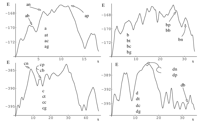
For each calculation we used the following settings: the initial image density was set to 10, the iteration density to 30, and the maximum number of attempts to connect any pair of minima was limited to three. If a connection failed for a particular pair of minima then up to two more attempts were allowed before moving to the pair with the next smallest separation. For the second and third attempts the number of images was increased by each time. The maximum number of EF optimisation steps was set to with an RMS force convergence criterion of . In Figure 2.9 every panel is labelled with the separation between the endpoints, the number of transition states in the final pathway, the number of DNEB runs required, and the total number of gradient calls.
Individual pathways involving a single transition state have been characterised using indices [152] such as
| (2.41) |
which is a measure of the number of atoms that participate in the rearrangement.∗ ∗A modification of this Stillinger and Weber’s participation index as well as a new cooperativity index will be presented in Chapter 3. Here and are the position vectors of atom in the starting and finishing geometries, respectively. The largest values are marked in Figure 2.9 next to the corresponding transition state. It is noteworthy that the pathways LJ and LJ both involve some highly cooperative steps, and the average value of is more than 12 for both of them.
We have found that it is usually easier to locate good transition state candidates for a multi-step path if the stationary points are separated by roughly equal distances, in terms of the integrated path length. Furthermore, it seems that more effort is needed to characterise a multi-step path when transition states involving very different path lengths are present. In such cases it is particularly beneficial to build up a complete path in stages. To further characterise this effect we introduce a path length asymmetry index defined as
| (2.42) |
where and are the two integrated path lengths corresponding to the two downhill steepest-descent paths from a given transition state. For example, in rearrangement LJ , five steps out of nine have .
Barrier asymmetry also plays a role in the accuracy of the tangent estimate, the image density required to resolve particular regions of the path, and in our selection process for transition state candidates, which is based on the condition .† To characterise this property we define a barrier asymmetry index, , as
| (2.43) |
where and are the barriers corresponding to the forward and reverse reactions, respectively. The test cases in Figure 2.9 include a variety of situations, with barrier asymmetry index ranging from to . The maximum values of and are shown next to the corresponding transition states in this figure.
We note that the total number of gradient evaluations required to produce the above paths could be reduced significantly by optimising the DNEB parameters or the connection strategy in each case. However, our objective was to find parameters that give reasonable results for a range of test cases, without further intervention.
An essential part of the connection algorithm is a mechanism to incorporate the information obtained in all the previous searches into the next one. For large endpoint separations guessing the initial pathway can be difficult, and there is a large probability of finding many irrelevant stationary points at the beginning of the calculation.
The connection algorithm described earlier uses one double-ended search per cycle. However, we have found that this approach can be overwhelmed by the abundance of stationary points and pathways for complicated rearrangements. We therefore introduce the idea of an unconnected pathway and make the connection algorithm more focused by allowing more than one double-ended search per cycle.
Before each cycle a decision must be made as to which minima to try and connect next. Various strategies can be adopted, for example, selection based on the order in which transition states were found [8], or, selection of minima with the minimal separation in Euclidean distance space [7]. However, when the endpoints are very distant in configuration space, neither of these approaches is particularly efficient. The number of possible connections that might be tried simply grows too quickly if the , and sets become large. However, the new algorithm described below seems to be very effective.
The modified connection algorithm we have used in the present work is based on a shortest path method proposed by Dijkstra [153, 154]. We can describe the minima that are known at the beginning of each connection cycle as a complete graph [155], , where is the set of all minima and is the set of all the edges between them. Edges are considered to exist between every pair of minima and , even if they are in different , or sets, and the weight of the edge is chosen to be a function of the minimum Euclidean distance between them [142]:
| (2.44) |
where is the number of times a pair was selected for a connection attempt, is the maximal number of times we may try to connect any pair of minima, and is the minimum Euclidean distance between and . should be a monotonically increasing function, such as . We denote the number of minima in the set , as , and the number of edges in the set as .
Using the Dijkstra algorithm [153, 154] and the weighted graph representation described above, it is possible to determine the shortest paths between any minima in the database. The source is selected to be one of the endpoints. Upon termination of the Dijkstra algorithm, a shortest path from one endpoint to the other is extracted. If the weight of this pathway is non-zero, it contains one or more ‘gaps’. Connection attempts are then made for every pair of adjacent minima in the pathway with non-zero using the DNEB approach [7].
The computational complexity of the Dijkstra algorithm is at worst , and the memory requirements scale in a similar fashion. The most appropriate data structure is a weighted adjacency matrix. For the calculations presented here, the single source shortest paths problem was solved at the beginning of each cycle, which took less than of the total execution time for the largest database encountered. We emphasise here that once an initial path has been found, the perturbations considered in typical discrete path sampling (DPS) calculations will generally involve attempts to connect minima that are separated by far fewer elementary rearrangements than the endpoints. It is also noteworthy that the initial path is unlikely to contribute significantly to the overall rate constant. Nevertheless, it is essential to construct such a path to begin the DPS procedure.
The nature of the definition of the weight function allows the Dijkstra algorithm to terminate whenever a second endpoint, or any minimum connected to that endpoint via a series of elementary rearrangements, is reached. This observation reduces the computational requirements by an amount that depends on the distribution of the minima in the database among the , and sets. One of the endpoints is always a member of the set, while the other is a member of set. Either one can be chosen as the source, and we have found it most efficient to select the one from the set with fewest members. However, this choice does not improve the asymptotic bounds of the algorithm.
Tryptophan zippers are stable fast-folding -hairpins designed by Cochran et al. [156], which have recently generated considerable interest [157, 158]. In the present work we have obtained native to denatured state rearrangement pathways for five tryptophan zippers: trpzip , trpzip , trpzip , trpzip -I and trpzip . The notation is adopted from the work of Du et al. [158]. All these peptides contain twelve residues, except for trpzip , which has sixteen. Tryptophan zippers , , and -I differ only in the sequence of the turn. Experimental measurements of characteristic folding times for these peptides have shed some light on the significance of the turn sequence in determining the stability and folding kinetics of peptides with the -hairpin structural motif [158].
To model these molecules we used a modified CHARMM19 force field [4], with symmetrised Asn, Gln and Tyr dihedral angle and Cter improper dihedral angle terms, to ensure that rotamers of these residues have the same energies and geometries. These changes to the standard CHARMM19 force field are described in detail in Appendix A. Another small modification concerned the addition of a non-standard amino acid, D-proline, which was needed to model trpzip . The implicit solvent model EEF1 was used to account for solvation [11], with a small change to the original implementation to eliminate discontinuities [159].
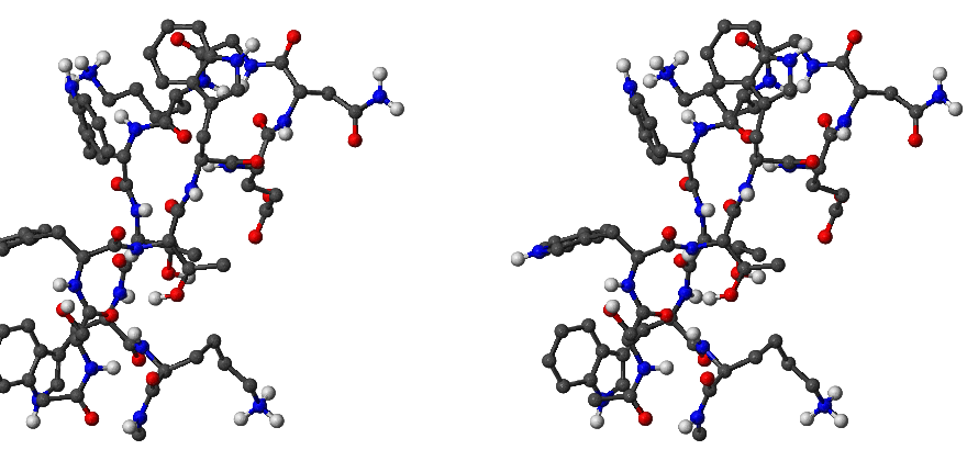
We have used the Dijkstra-based connection algorithm to obtain folding pathways for all five trpzip peptides. In each case the first endpoint was chosen to be the native state structure, which, for , and trpzips, was taken from the Protein Data Bank (PDB) [160]. There are no NMR structures available for and -I, so for these peptides the first endpoint was chosen to be the putative global minimum obtained using the basin-hopping method [161–163]. The folded state for trpzip is depicted in Figure 2.10. The total charge of this molecule is (two Lys)(Glu). However, in our calculations the total charge was zero because in the CHARMM19 force field ionic sidechains and termini are neutral when the EEF1 solvation model is used [11].
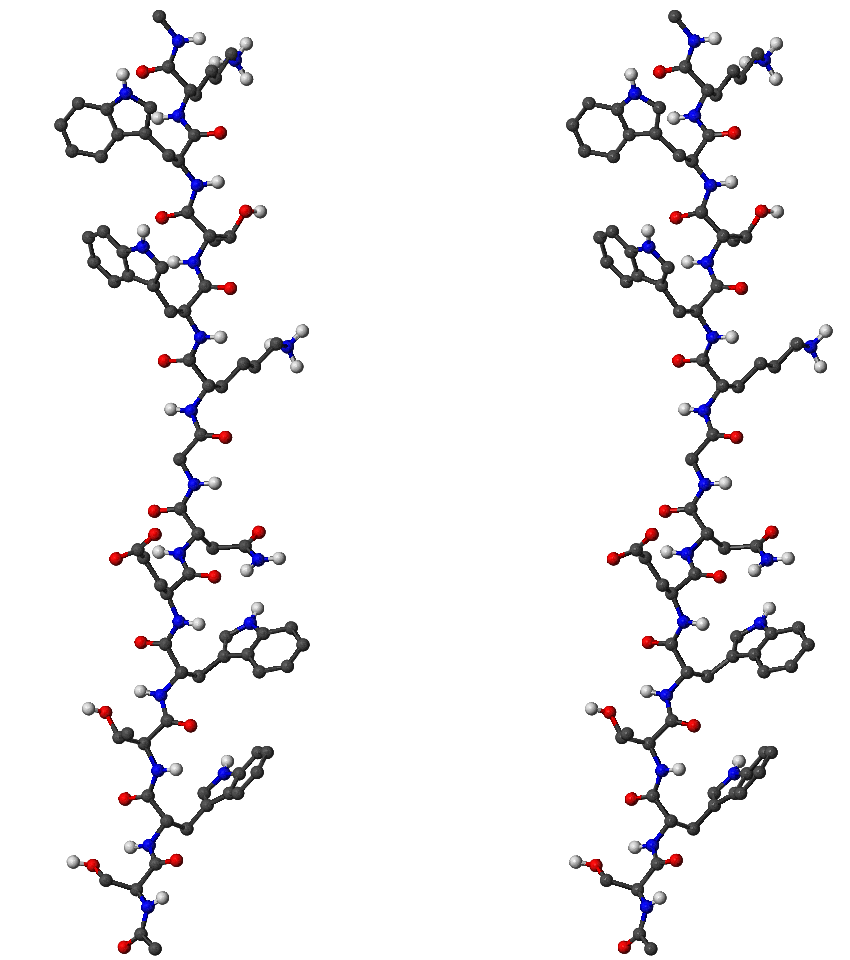
The second endpoint was chosen to be an extended structure, which was obtained by simply minimising the energy of a conformation with all the backbone dihedral angles set to 180 degrees. All the stationary points (including these obtained during the connection procedure) were tightly converged to reduce the root-mean-squared force below kcalmol Å. The unfolded state for trpzip is depicted in Figure 2.11 for example.
Each of the five trpzip pathway searches was conducted on a single Pentium 4 3.0GHz 512Mb cache CPU and required less than 24 hours of CPU time. The timings could certainly be improved by optimising the various parameters employed throughout the searches. However, it is more important that the connections actually succeed in a reasonably short time. It only requires one complete path to seed a DPS run, and we expect the DPS procedure to reduce the length of the initial path by a least a factor of two in sampling the largest contributions to the effective two-state rate constants. The results of all the trpzip calculations are shown in Figure 2.12.
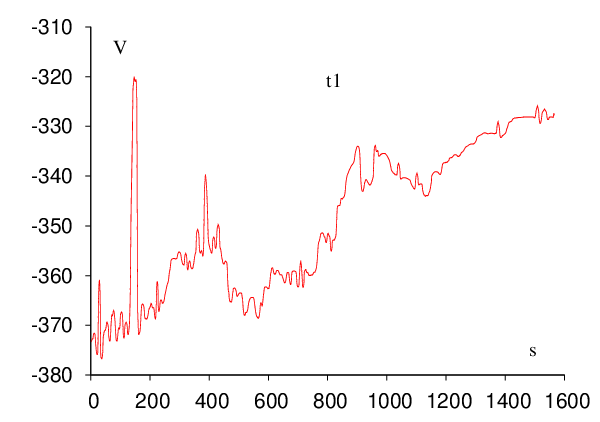
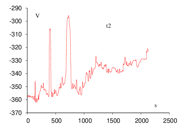
| Trpzip | Steps | Cycles | Searches | Points |
| 1 | 70 | 44 | 190 | 161,137 |
| 2 | 93 | 386 | 1325 | 761,626 |
| 3 | 128 | 203 | 703 | 565,487 |
| 3-I | 67 | 52 | 172 | 203,158 |
| 4 | 91 | 135 | 558 | 284,244 |
One of the two most important results of this chapter is probably the doubly nudged elastic band formulation, in which a portion of the spring gradient perpendicular to the path is retained. With this modification we found that L-BFGS minimisation of the images is stable, thus providing a significant improvement in efficiency. Constraints such as elimination of overall rotation and translation are not required, and the DNEB/L-BFGS method has proved to be reliable for relatively complicated cooperative rearrangements in a number of clusters.
In comparing the performance of the L-BFGS and quenched velocity Verlet (QVV) methods for optimising chains of images we have also investigated a number of alternative QVV schemes. We found that the best approach is to quench the velocity after the coordinate update, so that the velocity response to the new gradient lags one step behind the coordinate updates. However, this slow-response QVV (SQVV) method does not appear to be competitive with L-BFGS.
We have revised our previous scheme [8] for constructing connections between distant minima using multiple transition state searches. Previously we have used an NEB/L-BFGS framework for this purpose, with eigenvector-following refinement of transition state candidates and characterisation of the connected minima using energy minimised approximations to the steepest-descent paths [8, 133]. When the DNEB/L-BFGS approach is used we have found that it is better to spend more effort in the DNEB phase of the calculation, since a number of good transition state guesses can often be obtained even when the number of images is relatively small. In favourable cases a complete path linking the required endpoints may be obtained in one cycle. Of course, this was always the objective of the NEB approach [27–30], but we have not been able to achieve such results reliably for complex paths without the current modifications.
When a number of transition states are involved we still find it more efficient to build up the overall path in stages, choosing endpoints that become progressively closer in space. This procedure has been entirely automated within the OPTIM program, which can routinely locate complete paths for highly cooperative multi-step rearrangements, such as those connecting different morphologies of the LJ and LJ clusters.
For complex rearrangements the number of elementary steps involved may be rather large, and new methods for constructing an initial path are needed. This path does not need to be the shortest, or the fastest, but it does need to be fully connected. The second most important result of this chapter is probably a connection procedure based upon Dijkstra’s shortest path algorithm, which enables us to select the most promising paths that include missing connections for subsequent double-ended searches. We have found that this approach enables initial paths containing more than a hundred steps to be calculated automatically for a variety of systems. Results have been presented for trpzip peptides here and for buckminsterfullerene, the GB1 hairpin and the villin headpiece subdomain elsewhere [167]. These paths will be employed to seed future discrete path sampling calculations. This approach greatly reduces the computational demands of the method, and has allowed us to tackle more complicated problems. The new algorithm has also been implemented within our OPTIM program, and a public domain version is available for download from the Internet [138].