3 Properties of Rearrangement Pathways

Chapter 3
Properties of Rearrangement Pathways

2.5.6 A Revised Connection Algorithm
2.5.7 Applications to Isomerisation of LJ

_{38}

and LJ

_{75}

2.5.8 A Dijkstra-based Selector
2.5.9 Applications to Tryptophan Zippers
2.6 Summary

There is a difference between knowing
the path and walking the path.

Andy and Larry Wachowski, The Matrix

3.1 Introduction

The number of elementary rearrangements increases exponentially with system size as for the number of transition states. For instance, there are approximately 30,000 such pathways on the PES of the 13-atom cluster bound by the Lennard-Jones potential. When permutation-inversion isomers are included, this number increases by a factor of order $2 \times N!$ [9]. For PES’s that support such a large number of stationary points a whole range of properties is spanned by the corresponding rearrangement pathways. Understanding these properties can be helpful in answering questions such as why some rearrangement pathways are harder to find than others and whether there is any correlation between these properties that we could potentially utilise in studying PES’s.

Two activation barriers can be defined for each pathway in terms of the energy difference between the transition state and each of the minima. For non-degenerate rearrangements [9, 148] the two sides of the path are termed uphill and downhill, where the uphill barrier is the larger one, which leads to the higher minimum. The barriers and the normal modes of the minima and transition states can be used to calculate rate constants using harmonic transition state theory [45, 46, 48]. More sophisticated treatments based on anharmonic densities of states are possible but can be hard to reconcile with the coarse-grained view of the landscape adopted here, as a detailed knowledge of the basins of attraction is required [168, 169].

For each local minimum a catchment basin can be defined in terms of all the configurations from which steepest-descent paths lead to that minimum [170]. Some of these paths originate from transition states on the boundary of the catchment basin, which connect a given minimum to adjacent minima. The integrated path length for such rearrangements provides a measure of the separation between local minima, and may be related to the density of stationary points in configuration space. The integrated path length is usually approximated as the sum of Euclidean distances between configurations sampled along appropriate steepest-descent paths [9]. It provides a convenient coordinate for monitoring the progress of the reaction.

Calculated pathways can always be further classified mechanistically. For example, some rearrangements preserve the nearest-neighbour coordination shell for all the atoms. In previous studies of bulk models these cage-preserving pathways were generally found to outnumber the more localised cage-breaking processes, which are necessary for atomic transport [171]. It was found that the barriers for cage-breaking and cage-preserving processes were similar for bulk LJ systems, while the cage-breaking mechanisms have significantly higher barriers for bulk silicon modelled by the Stillinger-Weber potential [171].

For minima separated by increasing distances in configuration space, the pathways that connect them are likely to involve more and more elementary steps, and are not unique. Finding such paths in high-dimensional systems can become a challenging task [7, 8]. Some difficulties have been attributed to instabilities and inefficiencies in transition state searching algorithms [7, 107], as well as the existence of very different barrier height and path length scales [7]. A new algorithm for locating multi-step pathways in such cases was presented in the previous chapter.

In the present work we have used the doubly nudged elastic band (DNEB) method [7] in conjunction with eigenvector-following (EF) algorithms [12–24] to locate rearrangement pathways in various systems. The LJ potential was used to describe the $13$ - and $75$ -atom Lennard-Jones clusters, LJ $_{13}$ and LJ $_{75}$ . We have also considered a binary LJ (BLJ) system with parameters $σ_{A A} = 1.0$ , $σ_{B B} = 0.88$ , $σ_{A B} = 0.8$ , $𝜖_{A A} = 1.0$ , $𝜖_{B B} = 0.5$ , $𝜖_{A B} = 1.5$ , where $A$ and $B$ are atom types. The mixture with $A : B$ ratio $80 : 20$ provides a popular model bulk glass-former [171, 172]. We employed a periodically repeated cubic cell containing $205$ $A$ atoms and $51$ $B$ atoms. The density was fixed at $1.2 σ_{A A}^{- 3}$ and the Stoddard-Ford scheme was used to prevent discontinuities [173].

The motivation for this work was our observation that construction of some multi-step pathways using the connection algorithm described in Chapter 2 is particularly difficult. We were unable to relate these difficulties to simple properties of the pathways such as the integrated path length, the uphill and downhill barriers, or the barrier and path length asymmetries. Instead, more precise measures of localisation and cooperativity are required, as shown in the following sections. It also seems likely that such tools may prove useful in analysing the dynamics of supercooled liquids, where processes such as intrabasin oscillations and interbasin hopping have been associated with different rearrangement mechanisms [174]. In particular, cooperativity is believed to play an important role at low temperatures in glass-forming systems [175], and dynamic heterogeneity may result in decoupling between structural relaxation and transport properties for supercooled liquids [176].

3.2 Localisation

The outcome of a pathway calculation for an atomic system will generally be a set of intermediate geometries, and the corresponding energies, for points along the two unique steepest-descent paths that link a transition state to two local minima. This discrete representation is a convenient starting point for our analysis of localisation and cooperativity. We number the structures along the path $j = 1,$ starting from one of the two minima and reversing the other steepest-descent path, so that structure $N_{f}$ corresponds to the other minimum. The transition state then lies somewhere between frames $1$ and $N_{f}$ . We define the three-dimensional vector $r_{i} (j)$ to contain the Cartesian coordinates of atom $i$ for structure $j$ , i.e. $r_{i} (j) = (X_{i} (j), Y_{i} (j), Z_{i} (j))$ , where $X_{i} (j)$ is the $X$ coordinate of atom $i$ in structure $j$ , etc.

For each atom $i$ we also define the displacement between structures $j - 1$ and $j$ as

d_{i} (j) = | r_{i} (j) - r_{i} (j - 1) | .

(3.1)

Hence the sum of displacements

d_{i} = \sum_{j = 2}^{N_{f}} d_{i} (j),

(3.2)

is an approximation to the integrated path length for atom $i$ , which becomes increasingly accurate for smaller step sizes. The total integrated path length, $s$ , is approximated as

s = \sum_{j = 2}^{N_{f}} \sqrt{\sum_{i = 1}^{N} d_{i} {j)}^{2}},

(3.3)

where $N$ is the total number of atoms. $s$ is a characteristic property of the complete path, and is expected to correlate with parameters such as the curvature and barrier height for short paths [9, 177, 178].

The set ${d_{1}, d_{2}, \dots, d_{N}}$ containing all $N$ values of $d_{i}$ will be denoted ${d}$ , and analogous notation will be used for other sets below. We will also refer to the frequency distribution function, which can provide an alternative representation of such data [179]. For example, the frequency distribution function $ℱ$ for a given continuous variable, $x$ , tells us that $x$ occurs in a certain interval $ℱ (x)$ times.

Our objective in the present analysis is to provide a more detailed description of the degree of ‘localisation’ and ‘cooperativity’ corresponding to a given pathway. The first index we consider is $N_{p}$ , which is designed to provide an estimate of how many atoms participate in the rearrangement. We will refer to a rearrangement as localised if a small fraction of the atoms participate in the rearrangement, and as delocalised in the opposite limit. The second index we define, $N_{c}$ , is intended to characterise the number of atoms that move simultaneously, i.e. cooperatively. We will refer to a rearrangement as cooperative if most of the atoms that participate in the rearrangement move simultaneously, and as uncooperative otherwise.

The $n$ th moment about the mean for a data set ${x_{1}, x_{2}, . . ., x_{M}}$ is the expectation value of ${(x_{i} - ⟨ x ⟩)}^{n}$ , where $⟨ x ⟩ = \sum_{i = 1}^{M} x_{i} ∕ M$ and $M$ is the number of elements in the set. Hence for the set ${d}$ defined above we define the moments, $m_{n}$ , as

m_{n} = \frac{1}{N} \sum_{i = 1}^{N} {d_{i} - ⟨ d ⟩)}^{n} .

(3.4)

The kurtosis of the set ${d}$ is then defined as the dimensionless ratio

γ (d) = \frac{m_{4}}{{(m_{2})}^{2}},

(3.5)

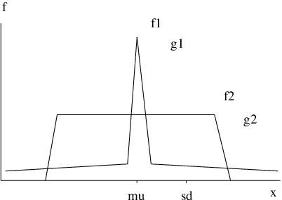
and provides a measure of the shape of the frequency distribution function corresponding to ${d}$ . If only one of the atoms moves, or all atoms except one move by the same amount, then $γ (d) = N$ . Alternatively, if half the atoms move by the same amount whilst the others are stationary, then $γ (d) = 1$ . Hence, a distribution with a broad peak and rapidly decaying tails will have a small kurtosis, $γ \sim 𝒪 (1)$ , while a distribution with a sharp peak and slowly decaying tails will have a larger value (Figure 3.1). The kurtosis can therefore identify distributions that contain large deviations from the average value [179]. For comparison, a Gaussian distribution has $γ = 3$ and a uniform distribution has $γ = 1.8$ .

Figure 3.1:Two frequency distribution functions $ℱ_{1}$ and $ℱ_{2}$ of a continuous variable $x$ are contrasted. Both functions have the same average $m_{1}^{'}$ and standard deviation ${\sqrt{m}}_{2}$ . However, due to the long tails, $ℱ_{1}$ has a significantly larger fourth moment $m_{4}$ and, hence, a larger kurtosis, $γ$ . If $γ > 3$ the distribution is said to be peaked or leptocurtic. Distributions with $γ > 3$ are known as platycurtic or heavy-tailed.

The above results show that the kurtosis $γ (d)$ can be used to quantify the degree of localisation or delocalisation of a given rearrangement. However, it has the serious disadvantage that highly localised and delocalised mechanisms both have large values of $γ (d)$ . Since we are interested in estimating the number of atoms that move relative to the number with small or zero displacements, a better approach is to use moments taken about the origin, rather than about the mean, i.e.

m_{n}^{'} = \frac{1}{N} \sum_{i = 1}^{N} d_{i}^{n},

(3.6)

following Stillinger and Weber [152]. Note that while $m_{1} = 0$ , the first moment $m_{1}^{'}$ is the mean value. We therefore estimate the number of atoms that participate in the rearrangement, $N_{p}$ , as

N_{p} = \frac{N}{γ^{'} (d)},

(3.7)

where

γ^{'} (d) = \frac{m_{4}^{'}}{{m_{2}^{'})}^{2}} .

(3.8)

For the system with $N$ atoms, if only one atom moves $N_{p} = 1$ , while if $K$ atoms move by the same amount, $N_{p} = K$ .

A similar index to $N_{p}$ has been employed in previous work [9, 19, 180] using only the displacements between the two local minima, which corresponds to taking $N_{f} = 2$ in Equation 3.2. Using $d_{i}$ values based upon a sum of displacements that approximates the integrated path length for atom $i$ , rather than the overall displacement between the two minima, better reflects the character of the rearrangement, as it can account for the nonlinearity of the pathway. To describe this property more precisely we introduce a pathway nonlinearity index defined by

α = \frac{s - D}{s},

(3.9)

where $D$ is the Euclidean distance between the endpoints,

D = \sqrt{\sum_{i = 1}^{N} {r_{i} (N_{f}) - r_{i} (1))}^{2}} .

(3.10)

We calculated the $α$ values for a database of 31,342 single transition state pathways of LJ $_{75}$ (hereafter referred to as the LJ $_{75}$ database). The average value of $α$ was $0.4$ with a standard deviation of $0.2$ , and, hence, there is a significant loss of information if $γ^{'}$ is calculated only from the endpoints using $N_{f} = 2$ . Comparison of the two indices for the LJ $_{75}$ database revealed many examples where neglect of intermediate structures produces a misleading impression of the number of atoms that move. The definition in Equation 3.7 is therefore suggested as an improvement on previous indices of localisation [9, 19, 152, 180].

3.3 Cooperativity

$N_{p}$ atoms can participate in a rearrangement according to a continuous range of cooperativity. At one end of the scale there are rearrangements where $N_{p}$ atoms all move simultaneously [see Figure 3.2 (a)]. Although these paths exhibit the highest degree of correlated atomic motion they do not usually pose a problem for double-ended transition state search algorithms [7, 30]. Linear interpolation between the two minima tends to generate initial guesses that lie close to the true pathway, particularly if $α \sim 0$ . At the opposite extreme, atoms can move almost one at a time, following a ‘domino’ pattern [see Figure 3.2 (b)]. Locating a transition state for such rearrangements may require a better initial guess, since linear interpolation effectively assumes that all the coordinates change at the same rate.

Figure 3.2:Comparison of cooperative (a) and uncooperative (b) rearrangements of the LJ $_{75}$ cluster, for mechanisms that are localised mainly on two atoms. The displacement $d$ as a function of the frame number $j$ is shown for the two atoms that move the most. Panels (c) and (d) illustrate the potential energy $V$ as a function of frame number $j$ for the rearrangements in (a) and (b), respectively. Dashed circles indicate flatter parts of the energy profile, which correspond to the most cooperative regions of the pathway.

The degree of correlation in the atomic displacements can be quantified by considering the displacement ‘overlap’

O_{k} = \sum_{j = 2}^{N_{f}} O_{k} j) = \sum_{j = 2}^{N_{f}} m i n [d_{c (1)} (j), d_{c (2)} (j), . . ., d_{c (k)} (j)],

(3.11)

where the index $k$ indicates that $O$ was calculated for $k$ atoms numbered $c (1)$ , $c (2)$ ,..., $c (k)$ . $c$ is a $k$ -dimensional vector that represents a particular choice of $k$ atoms from $N$ , and hence there are $C_{N}^{k} = N! ∕ k! (N - k)!$ possible values of $O_{k}$ . The index $O$ can be thought of as a measure of how the displacements of the atoms $c (1)$ , $c (2)$ , etc. overlap along the pathway. For example, if two atoms move at different times then $O_{2}$ is small for this pair because the minimum displacement in Equation 3.11 is always small. However, if both atoms move in the same region of the path then $O_{2}$ is larger.

We now explain how the statistics of the overlaps, $O_{k}$ , can be used to extract a measure of cooperativity (Figure 3.3). Suppose that $m$ atoms move simultaneously in a hypothetical rearrangement. Then all the overlaps $O_{k}$ for $k > m$ will be relatively small, because one or more atoms are included in the calculation whose motion is uncorrelated with the others. For overlaps $O_{k}$ with $k \leq m$ the set of $O_{k}$ for all possible choices of $k$ atoms from $N$ will exhibit some large values and some small. The large values occur when all the chosen atoms are members of the set that move cooperatively, while other choices give small values of $O_{k}$ . Hence the kurtosis of the set ${O_{k}}$ , $γ^{'} (O_{k})$ , calculated from moments taken about the origin, will be large for $k \leq m$ , and small for $k > m$ .

To obtain a measure of how many atoms move cooperatively we could therefore calculate $γ^{'} (O_{2})$ , $γ^{'} (O_{3})$ , etc. and look for the value of $k$ where $γ^{'} (O_{k})$ falls in magnitude. However, to avoid an arbitrary cut-off, it is better to calculate the kurtosis of the set ${γ^{'} (O_{2})$ , $γ^{'} (O_{3}), . . ., γ^{'} (O_{k})}$ , or $γ^{'} [γ^{'} (O)]$ for short. There are $N - 2$ members of this set, and by analogy with the definition of $N_{p} = N ∕ γ^{'} (d)$ , we could define a cooperativity index $N_{c} = (N - 2) ∕ γ^{'} [γ^{'} (O)] + 1$ . Then, if $γ^{'} (O_{2})$ is large, and all the other $γ^{'} (O_{k})$ are small, we obtain $γ^{'} (γ^{'} (O)) \sim N - 2$ and $N_{c} \sim 2$ , correctly reflecting the number of atoms that move together.

Figure 3.3: $γ^{'} (O_{2})$ plotted against $γ^{'} (d)$ for the LJ $_{75}$ pathway database. The figure shows how $γ^{'} (O_{2})$ can discriminate between rearrangements that have similar values of $γ^{'} (d)$ but different cooperativity. The data point for the most cooperative rearrangement localised on two atoms has $N_{p} = N_{c} = 2$ .

In practice, there are several problems with the above definition of $N_{c}$ . Calculating $N_{c}$ in this way quickly becomes costly as the number of atoms and/or number of frames in the pathway increases, because the number of elements in the set ${O_{k}}$ varies combinatorially with $k$ . Secondly, as $k$ approaches $N$ the distribution of all the possible values for $O_{k}$ becomes more and more uniform. Under these circumstances deviations from the mean that are negligible in comparison with the overall displacement can produce large kurtosises. Instead, we suggest a modified (and simpler) definition of $N_{c}$ , which better satisfies our objectives.

We first define the overlap of atomic displacements in a different manner. It can be seen from Equation 3.11 that the simultaneous displacement of $l$ atoms is included in each set of overlaps ${O_{k}}$ with $k \leq l$ . For example, if three atoms move cooperatively then both the ${O_{2}}$ and ${O_{3}}$ sets will include large elements corresponding to these contributions. Another redundancy is present within ${O_{k}}$ , since values in this set are calculated for all possible subsets of $k$ atoms and the displacement of each atom is therefore considered more than once. However, we can avoid this redundancy by defining a single $k -$ overlap, rather than dealing with $C_{N}^{k}$ different values.

Recall that $d_{i} (j)$ is the displacement of atom $i$ between frames $j - 1$ and $j$ . The ordering of the atoms is arbitrary but remains the same for each frame number $j$ . We now define $Δ_{i} (j)$ as the displacement of atom $i$ in frame $j$ , where index $i$ numbers the atoms in frame $j$ in descending order, according to the magnitude of $d_{i} (j)$ , e.g. atom $1$ in frame $2$ is now the atom with the maximum displacement between frames $1$ and $2$ , atom $2$ has the second largest displacement etc. As the ordering may vary from frame to frame, the atoms labelled $i$ in different frames can now be different. This relabelling greatly simplifies the notation we are about to introduce. Consider the $k$ -overlap defined as

Θ_{k} = \frac{1}{Δ_{t o t}} \sum_{j = 2}^{N_{f}} [Δ_{k} (j) - Δ_{k + 1} (j)],

(3.12)

where $k$ ranges from $1$ to $N$ , $Δ_{t o t} = \sum_{j = 2}^{N_{f}} Δ_{1} (j)$ and $Δ_{N + 1} (j)$ is defined to be zero for all $j$ . A schematic illustration of this construct is presented in Figure 3.4. For example, if only two atoms move in the course of the rearrangement, and both are displaced by the same amount (which may vary from frame to frame), the only non-zero overlap will be $Θ_{2}$ .

Figure 3.4:The $Θ$ indices for a hypothetical rearrangement localised on three atoms. For each of these atoms the displacement $d$ as a function of frame number $j$ is shown. The $d_{i}$ values in successive frames are connected with dotted ( $d_{1}$ ), dashed ( $d_{2}$ ) and solid ( $d_{3}$ ) lines. The corresponding contributions to $Θ_{1}$ , $Θ_{2}$ , and $Θ_{3}$ are shown as shaded squares and are labelled accordingly. If the remaining $N - 3$ atoms do not participate, and the area of one square is $S$ , the only non-zero overlaps will be $Θ_{1}$ , $Θ_{2}$ , and $Θ_{3}$ with values $5 ∕ 9$ , $3 ∕ 9$ and $1 ∕ 9$ , respectively.

We can now define an index to quantify the number of atoms that move cooperatively as

N_{c} = \sum_{k = 1}^{N} k Θ_{k} .

(3.13)

If only one atom moves during the rearrangement then $N_{c} = 1$ , while if $K$ atoms displace cooperatively during the rearrangement then $N_{c} = K$ . This definition is independent of the total displacement, the integrated path length, and the number of atoms, which makes it possible to compare $N_{c}$ indices calculated for different systems.

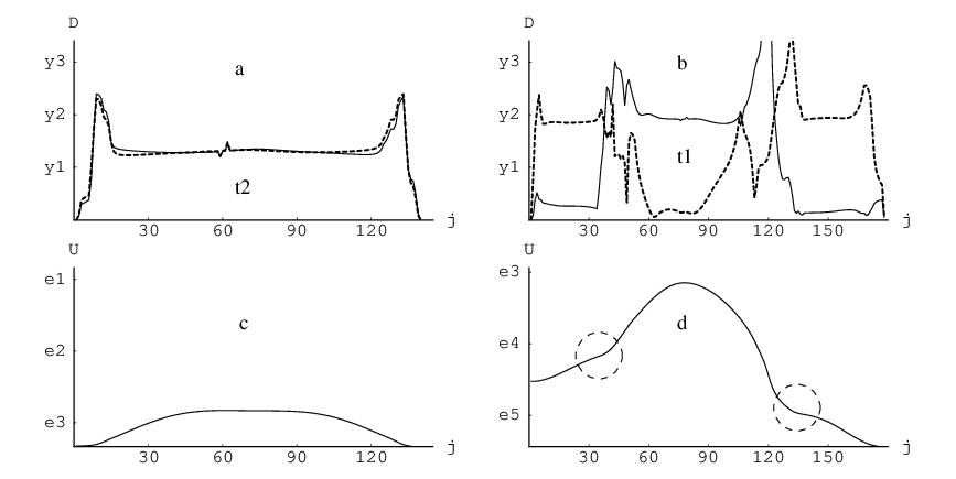
3.4 Applications to LJ $_{13}$ and LJ $_{75}$ Clusters and BLJ $_{256}$ Liquid

Figure 3.2 shows results for the most cooperative and uncooperative processes we have found for the LJ $_{75}$ cluster that are localised mainly on two atoms. In these calculations we have used the database of transition states that was found previously as the result of a discrete path sampling calculation conducted for this system [8, 10]. The cooperative rearrangement [Figure 3.2(a,c)] is the one with the maximum two-overlap $Θ_{2}$ . For this pathway $Θ_{2} = 0.7$ , $N_{p} = 3.4$ , and $N_{c} = 7.7$ . The values of $N_{p}$ and $N_{c}$ both reflect the fact that the motion of the two atoms is accompanied by a slight distortion of the cluster core. This example shows that while $N_{p}$ and $N_{c}$ allow us to quantify localisation and cooperativity, and correctly reflect the number of atoms that participate and move cooperatively in ideal cases, there will not generally be a simple correspondence between their values and the number of atoms that move. This complication is due to the fact that small displacements of atoms in the core will generally occur, no matter how localised the rearrangement is. In addition, the data reduction performed in Equation 3.7 and Equation 3.13 means that a range of pathways can give the same value for $N_{p}$ or $N_{c}$ . Since the size of the contribution from a large number of small displacements depends on the shape of the displacement distribution function the number of possibilities grows with the size of the index.

The uncooperative rearrangement depicted in the Figure 3.2(b,d) was harder to identify. In principle we could have selected the pathway that maximises $Θ_{1}$ from all the rearrangements localised on two atoms. However, this approach picks out rearrangements localised on one atom, where distortion of the core accounts for the value of $N_{p} > 1$ . Instead, we first selected from all the rearrangements with $N_{p} < 4$ those where two atoms move by approximately the same amount, while the displacement of any other atom is significantly smaller. These are the rearrangements that maximise $1 ∕ γ ({d_{1}, d_{2}})$ , where $d_{1}$ and $d_{2}$ are the total displacements of the two atoms that move the most. After this procedure we selected the rearrangement with the maximum value of $Θ_{1}$ . Figure 3.2 (b) shows that this rearrangement features the displacement of one atom at a time, and the atom that moves first also moves last. For this pathway the values of $Θ_{1}$ , $N_{p}$ and $N_{c}$ are $0.7$ , $3.8$ and $5.3$ , respectively. Further illustrations and movies of the corresponding rearrangements are available online [181].

Figure 3.2 illustrates several general trends that we have observed for cluster rearrangements. Firstly, we have found that the barrier height is smaller for the cooperative rearrangements [Figure 3.2(c,d)]. Usually atoms that move cooperatively are neighbours. Rearrangements generally involve a change of the environment for the atoms that move. Cooperative motion can reduce this perturbation since for any of the participants the local environment is partly preserved because it moves with the atom in question. Flatter points on the energy profile [circled in Figure 3.2(d)] usually signify a change in the mechanism, i.e. one group of atoms stops moving and another group starts. By comparing (b) and (d) in Figure 3.2 we conclude that flatter points on the energy profile correlate with the most cooperative parts of this rearrangement.

A simple correlation between barrier heights and $N_{p}$ and $N_{c}$ does not seem to exist. The barrier height is not a function of cooperativity alone, but also of the energetics of the participating atoms. The way the $N_{p}$ and $N_{c}$ indices have been defined can make them insensitive to details of the rearrangements that will affect the energetics. For instance, neither index depends on the location of the participating atoms or the directionality of their motion. In most cases cooperatively moving particles are adjacent, i.e. localised in space; however, long-distance correlations of atomic displacements also occur. One such case is depicted in Figure 3.5 (a). This path is nearly symmetric with respect to the integrated path length ( $π = 0.01$ ), but is very asymmetric with respect to the uphill and downhill barrier heights ( $β = 0.91$ ). This rearrangement has $N_{p} = N_{c} = 10$ . Interestingly, $N_{p}$ and $N_{c}$ calculated separately for both sides of the pathway are very similar, i.e. the two steepest-descent pathways cannot be distinguished using these indices. Close inspection of this rearrangement reveals that one side of the pathway involves the rearrangement of two atomic triplets that share a vertex, while the other side involves the drift of all five atoms on the surface of the cluster [see the insets in Figure 3.5 (a)]. Although $N_{c}$ does not distinguish these cases, the motion in the second side of the path is more cooperative. The participating atoms move together, which results in a significantly lower downhill barrier.

Figure 3.5:Two limitations of the cooperativity index $N_{c}$ . (a) $N_{c}$ is not sensitive to the spatial positions of the cooperatively moving atoms, nor to the directionality of their motion. The energy profile is depicted for a rearrangement of the LJ $_{75}$ cluster, which is very asymmetric with respect to barrier height but has similar integrated path lengths on either side of the transition state. The cooperativity index $N_{c}$ evaluated separately for the two sides is about $10$ in both cases. The motion of the five atoms that displace the most is shown schematically relative to a reference atom (black). (b) The displacement of two (left) and three (right) atoms $d$ as a function of the frame number $j$ is shown schematically for a hypothetical pathway. The rearrangement on the left is more cooperative because two atoms move together over a longer region of the path. However, the current definition of $N_{c}$ does not distinguish between these two cases.

$N_{p}$ and $N_{c}$ also describe properties of the whole pathway. A significant number of pathways that we observed were rather non-uniform, i.e. very cooperative phases alternated with uncooperative ones. To distinguish such pathways in the LJ $_{75}$ database we calculated a set ${N_{p}}$ containing $N_{p}$ ’s evaluated for each pair of adjacent frames. Then a selection of pathways was made with $m_{2} ∕ {(m_{1}^{'})}^{2} < 0.01$ , where $m_{2} ∕ {(m_{1}^{'})}^{2}$ is the moment ratio evaluated for the set ${N_{p}}$ . While this procedure ensured that $N_{p}$ corresponds closely to the number of atoms that moves between any two snapshots of the rearrangement, it did not distinguish cases where different atoms contribute to the value of $N_{p}$ in different frames [see Figure 3.5 (b)]. The average uphill and downhill barriers for this subset of rearrangements are $100$ times smaller than the average barriers for the complete LJ $_{75}$ database (Table 3.1). Figure 3.6 shows that $N_{p}$ and $N_{c}$ calculated for these rearrangements are highly correlated and span a range of values, implying that widely different pathways are represented. Finally, all the selected pathways are an order of magnitude shorter than the average path length for the whole database, even though this database contains many short rearrangements localised on one atom.

Table 3.1:Average uphill and downhill barriers, average integrated path length for the LJ

_{75}

rearrangement pathway database. Values are given for the whole database containing

31, 342

paths, and for a subset containing the

57

most cooperative paths. The units of energy and distance are

𝜖

and

σ

, respectively.



	All	Cooperative

Uphill barrier	3.03	0.06
Downhill barrier	0.97	0.03
Path length	3.08	0.58

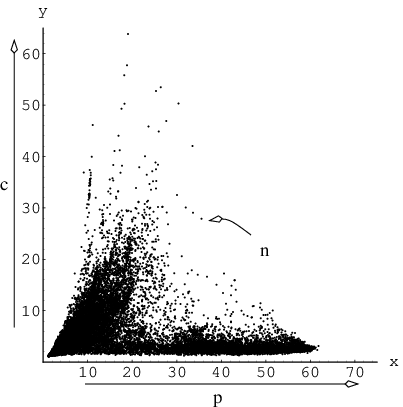
Figure 3.6: $N_{c}$ as a function of $N_{p}$ calculated for the $57$ most cooperative rearrangements from the LJ $_{75}$ pathway database.

Figure 3.7 shows the values of the $N_{p}$ and $N_{c}$ indices plotted against each other for pathway databases calculated for LJ $_{13}$ , LJ $_{75}$ and BLJ $_{256}$ . The two databases for BLJ $_{256}$ labelled as $1$ and $12$ are taken from Reference [171] and correspond to databases BLJ1 and BLJ12 in that paper. BLJ1 and BLJ12 were obtained using two different sampling schemes intended to provide an overview of a wide range of configuration space and a thorough probe of a smaller region, respectively. These databases were constructed by systematic exploration of the PES, and we refer the reader to the original work for further details [171]. Each BLJ $_{256}$ database contains $10, 000$ transition states. The LJ $_{13}$ and LJ $_{75}$ databases were obtained in discrete path sampling (DPS) studies [8, 10]. and contain $28, 756$ and $31, 342$ transition states, respectively. Figure 3.7 is a density plot where darker shading signifies a higher concentration of data points. The outlying points are connected by a solid line to define the area in which all the points lie. Figure 3.7 shows that as $N_{p}$ grows the allowed range of $N_{c}$ increases, especially for LJ $_{13}$ . For the LJ $_{75}$ database rearrangements with $N_{c} > N ∕ 2$ appear to be very rare or poorly sampled. Figure 3.7 also shows that for all these systems rearrangements localised on two or three atoms dominate. This result may be an intrinsic property. However, it may also be due to the geometric perturbation scheme used in producing the starting points for the transition state searches employed in generating these databases. For databases BLJ1 and BLJ12 there are significantly more rearrangements with larger values of $N_{p}$ and $N_{c}$ compared to LJ $_{75}$ , which suggests that the abundance of very localised rearrangements for clusters may be a surface effect. The apparent absence of cooperative rearrangements in LJ $_{75}$ database for large values of $N_{p}$ may be due to the fact that only the pathways between compact phases of this cluster were sampled thoroughly, i.e. rearrangements involving liquid-like structures that are expected to have larger values of $N_{c}$ are probably underrepresented.

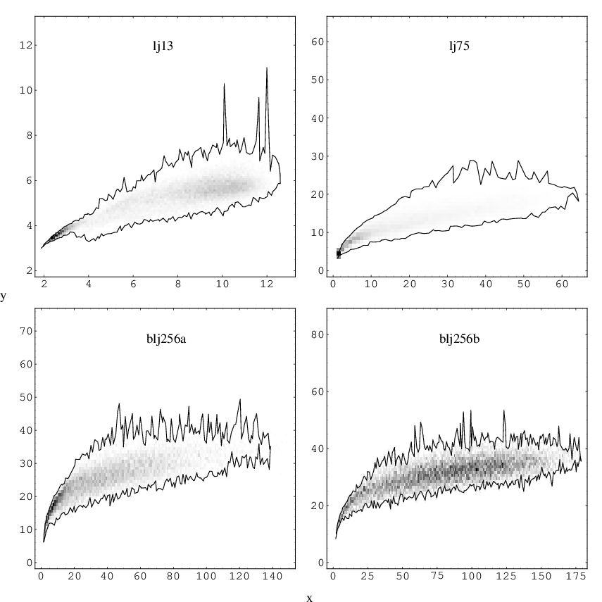
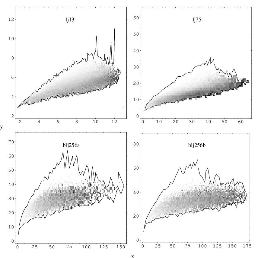
Figure 3.7: $N_{c}$ as a function of $N_{p}$ calculated from four pathway databases for LJ $_{13}$ , LJ $_{75}$ and BLJ $_{256}$ systems. Due to the large number of data points we employ a density plot, where the darkest shading corresponds to the highest concentration of points. Outlying points are connected to illustrate the boundaries of the data area. The two BLJ databases are taken from Reference [171].

Figure 3.8 depicts the average barrier as a function of the participation and cooperativity indices. $N_{p}$ and $N_{c}$ were calculated separately for both sides of the pathway and the corresponding barriers (uphill or downhill) were averaged to produce a density plot of barrier height. Data boundaries do not coincide with those shown in Figure 3.7 due to numerical imprecision in preparing Figure 3.7. Figure 3.8 illustrates that for each system cooperative rearrangements have the lowest barriers, irrespective of the value of $N_{p}$ . For clusters, cooperative rearrangements have lower barriers than uncooperative rearrangements with $N_{p}$ as small as $1 - 3$ , while for bulk barriers corresponding to rearrangements with low $N_{p}$ become comparable to these for very cooperative rearrangements with high $N_{p}$ .

Figure 3.8:Average barrier height as a function of $N_{p}$ and $N_{c}$ calculated for the same LJ $_{13}$ , LJ $_{75}$ and BLJ $_{256}$ pathway databases used in Figure 3.7. The indices were calculated separately for the two sides of each path. In this case the darkest shading corresponds to the highest barriers. Outlying points are connected to illustrate the boundaries of the data area. The two BLJ databases are taken from Reference [171].

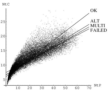
In further computational experiments we found that attempts to connect the endpoints of uncooperative pathways using the algorithm described in Chapter 2 either required more images and iterations or converged to an alternative pathway. In some cases additional difficulties arose, such as convergence to a higher index saddle instead of a transition state, which can happen if the linear interpolation guess conserves a symmetry plane. Figure 3.9 shows $N_{c}$ calculated from Equation 3.13 plotted against $N_{p}$ for the LJ $_{75}$ pathway database. Knowing the integrated path length, $s$ , for each pathway we started doubly nudged elastic band calculations with three images per unit of distance and $30$ iterations per image. Most of the points that correspond to runs that failed or converged to an alternative pathways are concentrated in the region of small values for $N_{c} ∕ N_{p}$ .

Figure 3.9: $N_{c}$ as a function of $N_{p}$ calculated for the LJ $_{75}$ pathway database. For each pathway we conducted DNEB calculations [7] assuming prior knowledge of the path. Every DNEB calculation employed $3 s$ images and $90 s$ iterations in each case, where $s$ is the integrated path length. Out of $31, 342$ DNEB runs $25, 158$ yielded a connected pathway while the rest did not (FAILED). Connected pathways are classified further as one-step pathways involving the correct transition state (OK) or an alternative transition state (ALT), or as multi-step pathways (MULTI), which involve more than one transition state. For each set of data points best fit straight lines obtained from linear regression are shown and labelled appropriately.

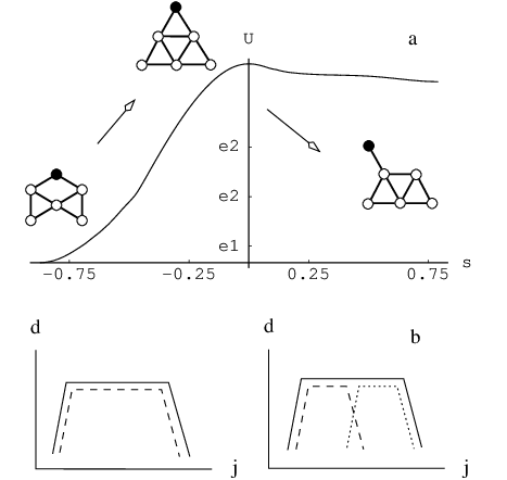
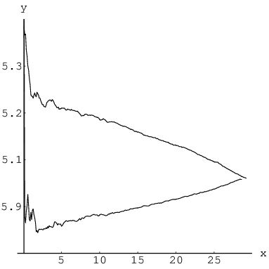
As can be seen from Figure 3.7, the LJ $_{13}$ database contains significantly more pathways with large values of $N_{p}$ and $N_{c}$ compared to LJ $_{75}$ , where most of the rearrangements are localised on two atoms. The fact that the LJ $_{13}$ database is almost exhaustive then suggests that localised rearrangements either start to dominate as the system size increases or that the sampling scheme used for LJ $_{75}$ was biased towards such mechanisms. Systematic sampling of the configuration space for stationary points often employs perturbations of every degree of freedom followed by minimisation [162]. The LJ $_{13}$ database was obtained in this fashion, while the LJ $_{75}$ database was generated during the DPS approach [8]. In this procedure discrete paths are perturbed by replacing local minima with structures obtained after perturbing all the coordinates and minimising. To investigate whether the perturbation scheme can affect the resulting database of stationary points in more detail we consider the case of LJ $_{13}$ , since nearly all the transition states are known. Figure 3.10 presents the results of two independent runs aimed at locating most of the transition states for this system. Every cycle a perturbation was applied to a randomly selected transition state from the database and the resulting geometry was used as a starting point for a new transition state search using eigenvector-following [19, 22–24, 72]. Only distinct permutation-inversion isomers were saved. In the first run (bottom curve) every degree of freedom was perturbed by $0.4 x$ , where $x$ is a random number in the interval $[- 1, 1]$ [162]. For the second run (top curve) we introduced a perturbation scheme including correlation. $2 \leq K \leq N ∕ 2$ atoms out of $N$ were displaced by a vector $0.4 (x_{1}, x_{2}, x_{3})$ , where the components $x_{1}$ , $x_{2}$ and $x_{3}$ are again random numbers drawn from $[- 1, 1]$ . The $K$ atoms to be displaced were selected based on their relative positions in the cluster. One atom was first selected at random, while the remaining $K - 1$ were chosen to be its closest neighbours. The top curve was generated from a run with $K = 6$ . Both runs required approximately the same time to produce two nearly identical databases, each containing about $29, 000$ pathways. However, as can be seen from Figure 3.7, random perturbation of all the degrees of freedom results in uncooperative rearrangements being found first, while employing correlated perturbations has the opposite effect.

Figure 3.10:The average value of $N_{c}$ for LJ $_{13}$ pathway databases as new paths are added. 6-atom correlated perturbations (top curve) and random perturbations of every degree of freedom (bottom curve) were used to produce starting points for refinement by eigenvector-following [19, 22–24, 72]. Average values were calculated every time $100$ new pathways were added.

3.5 Summary

The most important result of this chapter is probably the introduction of an index to quantify the cooperativity of atomic rearrangements. With this new measure it becomes possible to correlate cooperativity and barrier heights, and to show that cooperative rearrangements generally have lower barriers and shorter path lengths. We hope that these results will shed new light on relaxation mechanisms in complex systems, such as glasses and biomolecules, in future applications. For example, in a peptide or protein a large geometrical change can result from a rearrangement that could be described in terms of a single dihedral angle. In glasses and supercooled liquids an important research goal is to understand how observed dynamical properties, such as atomic diffusion and correlation functions [171, 174, 182, 183], are related to features of the underlying PES. The classification of elementary rearrangements as ‘cage-breaking’ or ‘cage-preserving’ [171, 184], and the emergence of structures such as ‘megabasins’ [171, 184–186] can now be investigated more precisely in terms of localisation and cooperativity.

We have also demonstrated that cooperative rearrangements are relatively easy to characterise using double-ended transition state searching algorithms, since linear interpolation produces an effective initial guess. Uncooperative rearrangements are usually harder to find using such methods, and alternative initial guesses may be helpful in these cases.

Single-ended transition state searching has been used both in conjunction with double-ended methods, and as a way to sample potential energy surfaces for stationary points. Stationary point databases constructed using random perturbations followed by quenching are likely to be biased towards uncooperative rearrangements. We have therefore outlined a strategy for generating initial guesses appropriate to single-ended transition state searching algorithms, which instead favours cooperative rearrangements. This approach also includes a parameter that is likely to influence the degree of localisation.

[next] [prev] [prev-tail] [front] [up]