4 Ensembles of Rearrangement Pathways

Chapter 4
Ensembles of Rearrangement Pathways

2.5.8 A Dijkstra-based Selector
2.5.9 Applications to Tryptophan Zippers
2.6 Summary

I dreamed a thousand new paths

\dots

I woke and walked my old one.

Chinese proverb

4.1 Introduction

Stochastic processes are widely used to treat phenomena with random factors and noise. Markov processes are an important class of stochastic processes for which future transitions do not depend upon how the current state was reached. Markov processes restricted to a discrete, finite, or countably infinite state space are called Markov chains [123, 187, 188]. The parameter that is used to number all the states in the state space is called the time parameter. Many interesting problems of chemical kinetics concern the analysis of finite-state samples of otherwise infinite state space [9].

When analysing the kinetic databases obtained from discrete path sampling (DPS) studies [8] it can be difficult to extract the phenomenological rate constants for processes that occur over very long time scales [9]. DPS databases are composed of local minima of the potential energy surface (PES) and the transition states that connect them. While minima correspond to mechanically stable structures, the transition states specify how these structures interconvert and the corresponding rates. Whenever the potential energy barrier for the event of interest is large in comparison with $k_{B} T$ the event becomes rare, where $T$ is the temperature and $k_{B}$ is Boltzmann’s constant.

The most important tools previously employed to extract kinetic information from a DPS stationary point database are the master equation [189], kinetic Monte Carlo [190, 191] (KMC) and matrix multiplication (MM) methods [8]. The system of linear master equations in its matrix formulation can be solved numerically to yield the time evolution of the occupation probabilities starting from an arbitrary initial distribution. This approach works well only for small problems, as the diagonalisation of the transition matrix, $P$ , scales as the cube of the number of states [9]. In addition, numerical problems arise when the magnitude of the eigenvalues corresponding to the slowest relaxation modes approaches the precision of the zero eigenvalue corresponding to equilibrium [192]. The KMC approach is a stochastic technique that is commonly used to simulate the dynamics of various physical and chemical systems, examples being formation of crystal structures [193], nanoparticle growth [194] and diffusion [195]. The MM approach provides a way to sum contributions to phenomenological two-state rate constants from pathways that contain progressively more steps. It is based upon a steady-state approximation, and provides the corresponding solution to the linear master equation [189, 196]. The MM approach has been used to analyse DPS databases in a number of systems ranging from Lennard-Jones clusters [8, 10] to biomolecules [133, 197].

Both the standard KMC and MM formulations provide rates at a computational cost that generally grows exponentially as the temperature is decreased. In this chapter we describe alternative methods that are deterministic and formally exact, where the computational requirements are independent of the temperature and the time scale on which the process of interest takes place.

4.1.1 Graph Theory Representation of a Finite-state Markov Chain

In general, to fully define a Markov chain it is necessary to specify all the possible states of the system and the rules for transitions between them. Graph theoretical representations of finite-state Markov chains are widely used [187, 198–200]. Here we adopt a digraph [154, 201] representation of a Markov chain, where nodes represent the states and edges represent the transitions of non-zero probability. The edge $e_{i, j}$ describes a transition from node $j$ to node $i$ and has a probability $P_{i, j}$ associated with it, which is commonly known as a routing or branching probability. A node can be connected to any number of other nodes. Two nodes of a graph are adjacent if there is an edge between them [202].

For digraphs all connections of a node are classified as incoming or outgoing. The total number of incoming connections is the in-degree of a node, while the total number of outgoing connections is the out-degree. In a symmetric digraph the in-degree and out-degree are the same for every node [154]. $AdjIn [i]$ is the set of indices of all nodes that are connected to node $i$ via incoming edges that finish at node $i$ . Similarly, $AdjOut [i]$ is the set of the indices of all the nodes that are connected to node $i$ via outgoing edges from node $i$ . The degree of a graph is the maximum degree of all of its nodes. The expectation value for the degree of an undirected graph is the average number of connections per node.

For any node $i$ the transition probabilities $P_{j, i}$ add up to unity,

\sum_{j} P_{j, i} = 1,

(4.1)

where the sum is over all $j \in AdjOut [i]$ . Unless specified otherwise all sums are taken over the set of indices of adjacent nodes or, since the branching probability is zero for non-adjacent nodes, over the set of all the nodes.

In a computer program dense graphs are usually stored in the form of adjacency matrices [154]. For sparse graphs [201] a more compact but less efficient adjacency-lists-based data structure exists [154]. To store a graph representation of a Markov chain, in addition to connectivity information (available from the adjacency matrix), the branching probabilities must be stored. Hence for dense graphs the most convenient approach is to store a transition probability matrix [187] with transition probabilities for non-existent edges set to zero. For sparse graphs, both the adjacency list and a list of corresponding branching probabilities must be stored.

4.1.2 The Kinetic Monte Carlo Method

The KMC method can be used to generate a memoryless (Markovian) random walk and hence a set of trajectories connecting initial and final states in a DPS database. Many trajectories are necessary to collect appropriate statistics. Examples of pathway averages that are usually obtained with KMC are the mean path length and the mean first passage time. Here the KMC trajectory length is the number of states (local minima of the PES in the current context) that the walker encounters before reaching the final state. The first passage time is defined as the time that elapses before the walker reaches the final state. For a given KMC trajectory the first passage time is calculated as the sum of the mean waiting times in each of the states encountered.

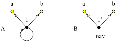
Within the canonical Metropolis Monte Carlo approach a step is always taken if the proposed move lowers the energy, while steps that raise the energy are allowed with a probability that decreases with the energy difference between the current and proposed states [32]. An efficient way to propagate KMC trajectories was suggested by Bortz, Kalos, and Lebowitz (BKL) [190]. According to the BKL algorithm, a step is chosen in such a way that the ratios between transition probabilities of different events are preserved, but rejections are eliminated. Figure 4.1 explains this approach for a simple discrete-time Markov chain. The evolution of an ordinary KMC trajectory is monitored by the ‘time’ parameter $n$ , $n \in 𝕎$ , which is incremented by one every time a transition from any state is made. The random walker is in state $1$ at time $n = 0$ . The KMC trajectory is terminated whenever an absorbing state is encountered. As $P_{1, 1}$ approaches unity transitions out of state $1$ become rare. To ensure that every time a random number is generated (one of the most time consuming steps in a KMC calculation) a move is made to a neighbouring state we average over the transitions from state $1$ to itself to obtain the Markov chain depicted in Figure 4.1 (b).

Figure 4.1:BKL algorithm for propagating a KMC trajectory applied to a three-state Markov chain. (a) The transition state diagram is shown where states and transitions are represented by circles and directed arrows, respectively. The Markov chain is parametrised by transition probabilities $P_{α, 1}$ , $P_{β, 1}$ and $P_{1, 1}$ . Absorbing states $α$ and $β$ are shaded. If $P_{1, 1}$ is close to unity the KMC trajectory is likely to revisit state $1$ many times before going to $α$ or $β$ . (b) State $1$ is replaced with state $1^{'}$ . The new Markov chain is parametrised by transition probabilities $P_{α, 1^{'}}$ , $P_{β, 1^{'}}$ and the average time for escape from state $1$ , $τ_{1}$ . Transitions from state $1^{'}$ to itself are forbidden. Every time state $1^{'}$ is visited the simulation ‘clock’ is incremented by $τ_{1}$ .

Transitions from state $1$ to itself can be modelled by a Bernoulli process [33] with the probability of success equal to $P_{1, 1}$ . The average time for escape from state $1$ is obtained as

τ_{1} = (1 - P_{1, 1}) \sum_{n = 0}^{\infty} (n + 1) {(P_{1, 1})}^{n} = \frac{1}{(1 - P_{1, 1})},

(4.2)

which can be used as a measure of the efficiency of trapping [203]. Transition probabilities out of state $1$ are renormalised:

\begin{matrix} P_{α, 1^{'}} & = & \frac{P_{α, 1}}{1 - P_{1, 1}}, \\ P_{β, 1^{'}} & = & \frac{P_{β, 1}}{1 - P_{1, 1}} . \end{matrix}

(4.3)

Similar ideas underlie the accelerated Monte Carlo algorithm suggested by Novotny [26]. According to this ‘Monte Carlo with absorbing Markov chains’ (MCAMC) method, at every step a Markov matrix, $P$ , is formed, which describes the transitions in a subspace $S$ that contains the current state $α$ , and a set of adjacent states that the random walker is likely to visit from $α$ . A trajectory length, $n$ , for escape from $S$ is obtained by bracketing a uniformly distributed random variable, $r$ , as

\sum_{β} {P^{n}]}_{β, α} < r \leq \sum_{β} {P^{n - 1}]}_{β, α} .

(4.4)

Then an $n$ -step leapfrog move is performed to one of the states $γ \notin S$ and the simulation clock is incremented by $n$ . State $γ$ is chosen at random with probability

{R P^{n - 1}]}_{γ, α} ∕ \sum_{γ} {R P^{n - 1}]}_{γ, α},

(4.5)

where $R_{γ, α}$ is the transition probability from state $α \in S$ to state $γ \notin S$ . Both the BKL and MCAMC methods can be many orders of magnitude faster than the standard KMC method when kinetic traps are present.

In chemical kinetics transitions out of a state are described using a Poisson process, which can be considered a continuous-time analogue of Bernoulli trials. The transition probabilities are determined from the rates of the underlying transitions as

P_{j, i} = \frac{k_{j, i}}{\sum_{α} k_{α, i}} .

(4.6)

There may be several escape routes from a given state. Transitions from any state to directly connected states are treated as competing independent Poisson processes, which together generate a new Poisson distribution [179]. $n$ independent Poisson processes with rates $k_{1}, k_{2}, k_{3}, \dots, k_{n}$ combine to produce a Poisson process with rate $k = \sum_{i = 1}^{n} k_{i}$ . The waiting time for a transition to occur to any connected state is then exponentially distributed as $k \exp (- kt)$ [204].

Given the exponential distribution of waiting times the mean waiting time in state $i$ before escape, $τ_{i}$ , is $1 ∕ \sum_{j} k_{j, i}$ and the variance of the waiting time is simply $τ_{i}^{2}$ . Here $k_{j, i}$ is the rate constant for transitions from $i$ to $j$ . When the average of the distribution of times is the property of interest, and not the distribution of times itself, it is sufficient to increment the simulation time by the mean waiting time rather than by a value drawn from the appropriate distribution [9, 205]. This modification to the original KMC formulation [206, 207] reduces the cost of the method and accelerates the convergence of KMC averages without affecting the results.

4.1.3 Discrete Path Sampling

The result of a DPS simulation is a database of local minima and transition states from the PES [8–10]. To extract thermodynamic and kinetic properties from this database we require partition functions for the individual minima and rate constants, $k_{α, β}$ , for the elementary transitions between adjacent minima $β$ and $α$ . We usually employ harmonic densities of states and statistical rate theory to obtain these quantities, but these details are not important here. To analyse the global kinetics we further assume Markovian transitions between adjacent local minima, which produces a set of linear (master) equations that governs the evolution of the occupation probabilities towards equilibrium [189, 196]

\frac{d P_{α} (t)}{dt} = \sum_{β} k_{α, β} P_{β} (t) - P_{α} (t) \sum_{β} k_{β, α},

(4.7)

where $P_{α} (t)$ is the occupation probability of minimum $α$ at time $t$ .

All the minima are classified into sets $A$ , $B$ and $I$ . When local equilibrium is assumed within the $A$ and $B$ sets we can write

P_{a} (t) = \frac{P_{a}^{eq} P_{A} (t)}{P_{A}^{eq}} and P_{b} (t) = \frac{P_{b}^{eq} P_{B} (t)}{P_{B}^{eq}},

(4.8)

where $P_{A} (t) = \sum_{a \in A} P_{a} (t)$ and $P_{B} (t) = \sum_{b \in B} P_{b} (t)$ . If the steady-state approximation is applied to all the intervening states $i \in I = {i_{1}, i_{2}, i_{3}, \dots, i_{n_{i}}}$ , so that

\frac{d P_{i} (t)}{dt} = 0,

(4.9)

then Equation 4.7 can be written as [9]

\begin{matrix} \frac{d P_{A} (t)}{dt} & = & k_{A, B} P_{B} (t) - k_{B, A} P_{A} (t), \\ \frac{d P_{B} (t)}{dt} & = & k_{B, A} P_{A} (t) - k_{A, B} P_{B} (t) . \end{matrix}

(4.10)

The rate constants $k_{A, B}$ and $k_{B, A}$ for forward and backward transitions between states $A$ and $B$ are the sums over all possible paths within the set of intervening minima of the products of the branching probabilities corresponding to the elementary transitions for each path:

\begin{matrix} k_{A, B}^{DPS} & = & \sum_{a \leftarrow b}^{'} \frac{k_{a, i_{1}}}{\sum_{α_{1}} k_{α_{1}, i_{1}}} \frac{k_{i_{1}, i_{2}}}{\sum_{α_{2}} k_{α_{2}, i_{2}}} \dots \frac{k_{i_{n - 1}, i_{n}}}{\sum_{α_{n}} k_{α_{n}, i_{n}}} \frac{k_{i_{n}, b} P_{b}^{eq}}{P_{B}^{eq}} \\ = & \sum_{a \leftarrow b}^{'} P_{a, i_{1}} P_{i_{1}, i_{2}} \dots P_{i_{n - 1}, i_{n}} \frac{k_{i_{n}, b} P_{b}^{eq}}{P_{B}^{eq}}, \end{matrix}

(4.11)

and similarly for $k_{B, A}$ [8]. The sum is over all paths that begin from a state $b \in B$ and end at a state $a \in A$ , and the prime indicates that paths are not allowed to revisit states in $B$ . In previous contributions [8, 10, 133, 197] this sum was evaluated using a weighted adjacency matrix multiplication (MM) method, which will be reviewed in Section 4.2.

4.1.4 KMC and DPS Averages

We now show that the evaluation of the DPS sum in Equation 4.11 and the calculation of KMC averages are two closely related problems.

For KMC simulations we define sources and sinks that coincide with the set of initial states $B$ and final states $A$ , respectively.^∗ Every cycle of KMC simulation involves the generation of a single KMC trajectory connecting a node $b \in B$ and a node $a \in A$ . A source node $b$ is chosen from set $B$ with probability $P_{b}^{eq} ∕ P_{B}^{eq}$ .

We can formulate the calculation of the mean first passage time from $B$ to $A$ in graph theoretical terms as follows. Let the digraph consisting of nodes for all local minima and edges for each transition state be $𝒢$ . The digraph consisting of all nodes except those belonging to region $A$ is denoted by $G$ . We assume that there are no isolated nodes in $𝒢$ , so that all the nodes in $A$ can be reached from every node in $G$ . Suppose we start a KMC simulation from a particular node $β \in G$ . Let $P_{α} (n)$ be the expected occupation probability of node $α$ after $n$ KMC steps, with initial conditions $P_{β} (0) = 1$ and $P_{α \neq β} (0) = 0$ . We further define an escape probability for each $α \in G$ as the sum of branching probabilities to nodes in $A$ , i.e.

ℰ_{α}^{G} = \sum_{a \in A} P_{a, α} .

(4.12)

KMC trajectories terminate when they arrive at an $A$ minimum, and the expected probability transfer to the $A$ region at the $n$ th KMC step is $\sum_{α \in G} ℰ_{α}^{G} P_{α} (n)$ . If there is at least one escape route from $G$ to $A$ with a non-zero branching probability, then eventually all the occupation probabilities in $G$ must tend to zero and

Σ_{β}^{G} = \sum_{n = 0}^{\infty} \sum_{α \in G} ℰ_{α}^{G} P_{α} (n) = 1 .

(4.13)

We now rewrite $P_{α} (n)$ as a sum over all $n$ -step paths that start from $β$ and end at $α$ without leaving $G$ . Each path contributes to $P_{α} (n)$ according to the appropriate product of $n$ branching probabilities, so that

\begin{matrix} Σ_{β}^{G} & = & \sum_{α \in G} ℰ_{α}^{G} \sum_{n = 0}^{\infty} P_{α} (n) \\ = & \sum_{α \in G} ℰ_{α}^{G} \sum_{n = 0}^{\infty} \sum_{Ξ (n)} P_{α, i_{n - 1}} P_{i_{n - 1}, i_{n - 2}} \dots P_{i_{2}, i_{1}} P_{i_{1}, β} \\ = & \sum_{α \in G} ℰ_{α}^{G} 𝒮_{α, β}^{G} = 1, \end{matrix}

(4.14)

where $Ξ (n)$ denotes the set of $n$ -step paths that start from $β$ and end at $α$ without leaving $G$ , and the last line defines the pathway sum $𝒮_{α, β}^{G}$ .

It is clear from the last line of Equation 4.14 that for fixed $β$ the quantities $ℰ_{α}^{G} 𝒮_{α, β}^{G}$ define a probability distribution. However, the pathway sums $𝒮_{α, β}^{G}$ are not probabilities, and may be greater than unity. In particular, $𝒮_{β, β}^{G} \geq 1$ because the path of zero length is included, which contributes one to the sum. Furthermore, the normalisation condition on the last line of Equation 4.14 places no restriction on $𝒮_{α, β}^{G}$ terms for which $ℰ_{α}^{G}$ vanishes.

We can also define a probability distribution for individual pathways. Let $𝒲_{ξ}$ be the product of branching probabilities associated with a path $ξ$ so that

𝒮_{α, β}^{G} = \sum_{n = 0}^{\infty} \sum_{ξ \in Ξ (n)} 𝒲_{ξ} \equiv \sum_{ξ \in α \leftarrow β} 𝒲_{ξ},

(4.15)

where $α \leftarrow β$ is the set of all appropriate paths from $β$ to $α$ of any length that can visit and revisit any node in $G$ . If we focus upon paths starting from minima in region $B$

\sum_{b \in B} \frac{P_{b}^{eq}}{P_{B}^{eq}} \sum_{α \in G} ℰ_{α}^{G} \sum_{ξ \in α \leftarrow b} 𝒲_{ξ} = \sum_{b \in B} \frac{P_{b}^{eq}}{P_{B}^{eq}} \sum_{α \in G_{A}} ℰ_{α}^{G} \sum_{ξ \in α \leftarrow b} 𝒲_{ξ} = 1,

(4.16)

where $G_{A}$ is the set of nodes in $G$ that are adjacent to $A$ minima in the complete graph $𝒢$ , since $ℰ_{α}^{G}$ vanishes for all other nodes. We can rewrite this sum as

\sum_{ξ \in G_{A} \leftarrow B} \frac{P_{b}^{eq}}{P_{B}^{eq}} ℰ_{α}^{G} 𝒲_{ξ} = \sum_{ξ \in A \leftarrow B} \frac{P_{b}^{eq}}{P_{B}^{eq}} 𝒲_{ξ} = \sum_{ξ \in A \leftarrow B} 𝒫_{ξ} = 1,

(4.17)

which defines the non-zero pathway probabilities $𝒫_{ξ}$ for all paths that start from any node in set $B$ and finish at any node in set $A$ . The paths $ξ \in A \leftarrow B$ can revisit any minima in the $G$ set, but include just one $A$ minimum at the terminus. Note that $𝒲_{ξ}$ and $𝒫_{ξ}$ can be used interchangeably if there is only one state in set $B$ .

The average of some property, $Q_{ξ}$ , defined for each KMC trajectory, $ξ$ , can be calculated from the $𝒫_{ξ}$ as

Q_{ξ}> = \sum_{ξ \in A \leftarrow B} 𝒫_{ξ} Q_{ξ} .

(4.18)

Of course, KMC simulations avoid this complete enumeration by generating trajectories with probabilities proportional to $𝒫_{ξ}$ , so that a simple running average can be used to calculate $Q_{ξ}>$ . In the following sections we will develop alternative approaches based upon evaluating the complete sum, which become increasingly efficient at low temperature. We emphasise that these methods are only applicable to problems with a finite number of states, which are assumed to be known in advance.

The evaluation of the DPS sum defined in Equation 4.11 can also be rewritten in terms of pathway probabilities:

\begin{matrix} k_{A, B}^{DPS} & = & \sum_{n = 0}^{\infty} \sum_{Ξ (n)}^{'} P_{α, i_{1}} P_{i_{1}, i_{2}} \dots P_{i_{n - 1}, i_{n}} \frac{k_{i_{n}, β} P_{β}^{eq}}{P_{B}^{eq}}, \\ = & \sum_{n = 0}^{\infty} \sum_{Ξ (n)}^{'} P_{α, i_{1}} P_{i_{1}, i_{2}} \dots P_{i_{n - 1}, i_{n}} P_{i_{n}, β} τ_{β}^{- 1} \frac{P_{β}^{eq}}{P_{B}^{eq}} \\ = & \sum_{ξ \in A \leftarrow B}^{'} 𝒫_{ξ} τ_{β}^{- 1}, \end{matrix}

(4.19)

where the prime on the summation indicates that the paths are not allowed to revisit the $B$ region. We have also used the fact that $k_{i_{n}, b} = P_{i_{n}, b} ∕ τ_{b}$ .

A digraph representation of the restricted set of pathways defined in Equation 4.19 can be created if we allow sets of sources and sinks to overlap. In that case all the nodes $A \cup B$ are defined to be sinks and all the nodes in $B$ are the sources, i.e. every node in set $B$ is both a source and a sink. The required sum then includes all the pathways that finish at sinks of type $A$ , but not those that finish at sinks of type $B$ . The case when sets of sources and sinks (partially) overlap is discussed in detail in Section 4.6.

4.1.5 Mean Escape Times

Since the mean first passage time between states $B$ and $A$ , or the escape time from a subgraph, is of particular interest, we first illustrate a means to derive formulae for these quantities in terms of pathway probabilities.

The average time taken to traverse a path $ξ = α_{1}, α_{2}, α_{3}, \dots, α_{l (ξ)}$ is calculated as $𝔱_{ξ} = τ_{α_{1}} + τ_{α_{2}} + τ_{α_{3}}, \dots, τ_{α_{l (ξ) - 1}}$ , where $τ_{α}$ is the mean waiting time for escape from node $α$ , as above, $α_{k}$ identifies the $k$ th node along path $ξ$ , and $l (ξ)$ is the length of path $ξ$ . The mean escape time from a graph $G$ if started from node $β$ is then

𝒯_{β}^{G} = \sum_{ξ \in A \leftarrow β} 𝒫_{ξ} 𝔱_{ξ} .

(4.20)

If we multiply every branching probability, $P_{α, β}$ , that appears in $𝒫_{ξ}$ by $\exp (ζ τ_{β})$ then the mean escape time can be obtained as:

\begin{matrix} 𝒯_{β}^{G} & = & {\frac{d}{dζ} \sum_{ξ \in A \leftarrow β} P_{α_{l (ξ)}, α_{l (ξ) - 1}} e^{ζ τ_{l (ξ) - 1}} P_{α_{l (ξ) - 1}, α_{l (ξ) - 2}} e^{ζ τ_{l (ξ) - 2}} \dots P_{α_{2}, α_{1}} e^{ζ τ_{α_{1}}})]}_{ζ = 0} \\ = & {\frac{d}{dζ} \sum_{ξ \in A \leftarrow β} P_{α_{l (ξ)}, α_{l (ξ) - 1}} P_{α_{l (ξ) - 1}, α_{l (ξ) - 2}} \dots P_{α_{2}, α_{1}} e^{ζ 𝔱_{ξ}})]}_{ζ = 0} \\ = & \sum_{ξ \in A \leftarrow β} 𝒫_{ξ} 𝔱_{ξ} . \end{matrix}

(4.21)

This approach is useful if we have analytic results for the total probability $Σ_{β}^{G}$ , which may then be manipulated into formulae for $𝒯_{β}^{G}$ , and is standard practice in probability theory literature [208, 209]. The quantity $P_{α, β} e^{ζ τ_{β}}$ is similar to the ‘ $ζ$ probability’ described in Reference [208]. Analogous techniques are usually employed to obtain $𝒯_{β}^{G}$ and higher moments of the first-passage time distribution from analytic expressions for the first-passage probability generating function (see, for example, References [210, 211]). We now define ${\tilde{P}}_{α, β} = P_{α, β} e^{ζ τ_{β}}$ and the related quantities

\begin{matrix} {\tilde{ℰ}}_{α}^{G} & = & \sum_{a \in A} {\tilde{P}}_{a, α} = ℰ_{α}^{G} e^{ζ τ_{α}}, \\ {\tilde{𝒲}}_{ξ} & = & {\tilde{P}}_{α_{l (ξ)}, α_{l (ξ) - 1}} {\tilde{P}}_{α_{l (ξ) - 1}, α_{l (ξ) - 2}} \dots {\tilde{P}}_{α_{2}, α_{1}} = 𝒲_{ξ} e^{ζ 𝔱_{ξ}}, \\ {\tilde{𝒫}}_{ξ} & = & {\tilde{𝒲}}_{ξ} P_{b}^{eq} ∕ P_{B}^{eq}, \\ {\tilde{𝒮}}_{α, β}^{G} & = & \sum_{ξ \in α \leftarrow β} {\tilde{𝒲}}_{ξ}, \\ and {\tilde{Σ}}_{β}^{G} & = & \sum_{α \in G} {\tilde{ℰ}}_{α}^{G} {\tilde{𝒮}}_{α, β}^{G} . \end{matrix}

(4.22)

Note that ${{\tilde{ℰ}}_{α}^{G}]}_{ζ = 0} = ℰ_{α}^{G}$ etc., while the mean escape time can now be written as

𝒯_{β}^{G} = {\frac{d {\tilde{Σ}}_{β}^{G}}{dζ}]}_{ζ = 0} .

(4.23)

In the remaining sections we show how to calculate the pathway probabilities, $𝒫_{ξ}$ , exactly, along with pathway averages, such as the waiting time. Chain graphs are treated in Section 4.2 and the results are generalised to arbitrary graphs in Section 4.3.

4.2 Chain Graphs

A general account of the problem of the first passage time in chemical physics was given by Weiss as early as 1965 [212]. In Reference [212] he summarised various techniques for solving such problems to date, and gave a general formula for moments of the first passage time in terms of the Green’s function of the Fokker-Plank operator. Explicit expressions for the mean first passage times in terms of the basic transition probabilities for the case of a one-dimensional random walk were obtained by Ledermann and Reuter in 1954 [213], Karlin and MacGregor in 1957 [214], Weiss in 1965 [212], Gardiner in 1985 [215], Van den Broeck in 1988 [216], Le Doussal in 1989 [217], Murthy and Kehr and Matan and Havlin in 1989-1990 [211, 218, 219], Raykin in 1992 [210], Bar-Haim and Klafter in 1998 [203], Pury and Cáceres in 2003 [220], and Slutsky, Kardar and Mirny in 2004 [221, 222]. The one-dimensional random walk is therefore a very well researched topic, both in the field of probability and its physical and chemical applications. The results presented in this section differ in the manner of presentation.

A random walk in a discrete state space $S$ , where all the states can be arranged on a linear chain in such a way that $P_{i, j} = 0$ for all $| i - j | > 1$ , is called a one-dimensional or simple random walk (SRW). The SRW model attracts a lot of attention because of its rich behaviour and mathematical tractability. A well known example of its complexity is the anomalous diffusion law discovered by Sinai [223]. He showed that there is a dramatic slowing down of an ordinary power law diffusion (RMS displacement is proportional to ${(\log t)}^{2}$ instead of $t^{1 ∕ 2}$ ) if a random walker at each site $i$ experiences a random bias field $B_{i} = P_{i, i + 1} - P_{i, i - 1}$ . Stanley and Havlin generalised the Sinai model by introducing long-range correlations between the bias fields on each site and showed that the SRW can span a range of diffusive properties [224].

Although one-dimensional transport is rarely found on the macroscopic scale at a microscopic level there are several examples, such as kinesin motion along microtubules [225, 226], or DNA translocation through a nanopore [227, 228], so the SRW is interesting not only from a theoretical standpoint. There is a number of models that build upon the SRW that have exciting applications, examples being the SRW walk with branching and annihilation [229], and the SRW in the presence of random trappings [230]. Techniques developed for the SRW were applied to study more complex cases, such as, for example, multistage transport in liquids [231], random walks on fractals [232, 233], even-visiting random walks [234], self-avoiding random walks [235], random walks on percolation clusters [236, 237], and random walks on simple regular lattices [238, 239] and superlattices [240].

A presentation that discusses SRW first-passage probabilities in detail sufficient for our applications is that of Raykin [210]. He considered pathway ensembles explicitly and obtained the generating functions for the occupation probabilities of any lattice site for infinite, half-infinite and finite one-dimensional lattices with the random walker starting from an arbitrary lattice site. As we discuss below, these results have a direct application to the evaluation of the DPS rate constants augmented with recrossings. We have derived equivalent expressions for the first-passage probabilities independently, considering the finite rather than the infinite case, which we discuss in terms of chain digraphs below.

We define a chain as a digraph $C_{N} = (V, E)$ with $N$ nodes and $2 (N - 1)$ edges, where $V = {v_{1}, v_{2}, \dots, v_{N}}$ and $E = {e_{1, 2}, e_{2, 1}, e_{2, 3}, e_{3, 2}, \dots, e_{N - 2, N - 1}, e_{N - 1, N - 2}}$ . Adjacent nodes in the numbering scheme are connected via two oppositely directed edges, and these are the only connections. A transition probability $P_{α, β}$ is associated with every edge $e_{α, β}$ , as described in Section 4.1.1. An $N$ -node chain is depicted in Figure 4.2 as a subgraph of another graph.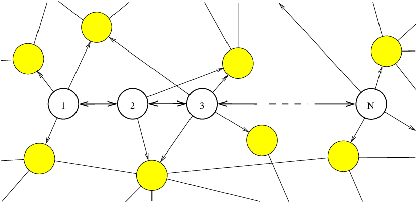

Figure 4.2:Chain graph of length $N$ , depicted as the subgraph of a larger graph. Visible sink nodes are shaded. Double-headed arrows represent pairs of directed edges.

The total probability of escape from the chain via node $N$ if started from node $1$ is of interest because it has previously been used to associate contributions to the total rate constant from unique paths in DPS studies [8, 9]. We can restrict the sampling to paths without recrossings between intermediate minima if we perform the corresponding recrossing sums explicitly [8].

We denote a pathway in $C_{N}$ by the ordered sequence of node indices. The length of a pathway is the number of edges traversed. For example, the pathway $1, 2, 1, 2, 3, 2, 3$ has length $6$ , starts at node $1$ and finishes at node $3$ . The indices of the intermediate nodes $2, 1, 2, 3, 2$ are given in the order in which they are visited. The product of branching probabilities associated with all edges in a path was defined above as $𝒲_{ξ}$ . For example, the product for the above pathway is $P_{3, 2} P_{2, 3} P_{3, 2} P_{2, 1} P_{1, 2} P_{2, 1}$ , which we can abbreviate as $𝒲_{3, 2, 3, 2, 1, 2, 1}$ . For a chain graph $C_{N}$ , which is a subgraph of $𝒢$ , we also define the set of indices of nodes in $𝒢$ that are adjacent to nodes in $C_{N}$ but not members of $C_{N}$ as $Adj [C_{N}]$ . These nodes will be considered as sinks if we are interested in escape from $C_{N}$ .

Analytical results for $C_{3}$ are easily derived:

\begin{matrix} 𝒮_{1, 1}^{C_{3}} & = \sum_{n = 0}^{\infty} {𝒲_{1, 2, 1} \sum_{m = 0}^{\infty} {𝒲_{2, 3, 2})}^{m})}^{n} & = \frac{1 - 𝒲_{2, 3, 2}}{1 - 𝒲_{1, 2, 1} - 𝒲_{2, 3, 2}}, \\ 𝒮_{2, 1}^{C_{3}} & = \sum_{n = 0}^{\infty} {𝒲_{2, 3, 2})}^{n} P_{2, 1} 𝒮_{1, 1}^{C_{3}} & = \frac{P_{2, 1}}{1 - 𝒲_{1, 2, 1} - 𝒲_{2, 3, 2}}, \\ 𝒮_{3, 1}^{C_{3}} & = P_{3, 2} \sum_{n = 0}^{\infty} {𝒲_{2, 3, 2})}^{n} P_{2, 1} 𝒮_{1, 1}^{C_{3}} & = \frac{𝒲_{3, 2, 1}}{1 - 𝒲_{1, 2, 1} - 𝒲_{2, 3, 2}}, \\ 𝒮_{2, 2}^{C_{3}} & = \sum_{n = 0}^{\infty} {𝒲_{1, 2, 1} + 𝒲_{2, 3, 2})}^{n} & = \frac{1}{1 - 𝒲_{1, 2, 1} - 𝒲_{2, 3, 2}}, \\ 𝒮_{3, 2}^{C_{3}} & = P_{3, 2} 𝒮_{2, 2}^{C_{3}} & = \frac{P_{3, 2}}{1 - 𝒲_{1, 2, 1} - 𝒲_{2, 3, 2}} . \end{matrix}

(4.24)

These sums converge if the cardinality of the set $Adj [C_{3}]$ is greater than zero. To prove this result consider a factor, $f$ , of the form

f = P_{α, β} P_{β, α} \sum_{m = 0}^{\infty} {(P_{β, γ} P_{γ, β})}^{m},

(4.25)

and assume that the branching probabilities are all non-zero, and that there is at least one additional escape route from $α$ , $β$ or $γ$ . We know that $P_{β, γ} P_{γ, β} < P_{γ, β} < 1$ because $P_{α, β} + P_{γ, β} \leq 1$ and $P_{α, β} \neq 0$ . Hence $f = P_{α, β} P_{β, α} ∕ (1 - P_{β, γ} P_{γ, β})$ . However, $P_{α, β} P_{β, α} + P_{β, γ} P_{γ, β} \leq P_{α, β} + P_{γ, β} \leq 1$ , and equality is only possible if $P_{β, α} = P_{β, γ} = P_{α, β} + P_{γ, β} = 1$ , which contradicts the assumption of an additional escape route. Hence $P_{α, β} P_{β, α} < 1 - P_{β, γ} P_{γ, β}$ and $f < 1$ . The pathway sums $𝒮_{1, 2}^{C_{3}}$ , $𝒮_{1, 3}^{C_{3}}$ , $𝒮_{2, 3}^{C_{3}}$ and $𝒮_{3, 3}^{C_{3}}$ can be obtained from Equation 4.24 by permuting the indices. The last two sums in Equation 4.24 are particularly instructive: the $n$ ’th term in the sum for $𝒮_{2, 2}^{C_{3}}$ and the $n$ ’th term in the sum for $𝒮_{3, 2}^{C_{3}}$ are the contributions from pathways of length $2 n$ and $2 n + 1$ , respectively.

The pathway sums $𝒮_{α, β}^{C_{N}}$ can be derived for a general chain graph $C_{N}$ in terms of recursion relations, as shown in Appendix C. The validity of our results for $C_{N}$ was verified numerically using the matrix multiplication method described in Reference [8]. For a chain of length $N$ we construct an $N \times N$ transition probability matrix $P$ with elements

P = \begin{matrix} 0 & P_{1, 2} & 0 & \dots \\ P_{2, 1} & 0 & P_{2, 3} & \dots \\ 0 & P_{3, 2} & 0 \\ ⋮ & ⋮ & ⋱ \end{matrix}) .

(4.26)

The matrix form of the system of Chapman-Kolmogorov equations [187] for homogeneous discrete-time Markov chains [123, 187] allows us to obtain the $n$ -step transition probability matrix recursively as

P (n) = PP (n - 1) = P^{n} .

(4.27)

$𝒮_{α, β}^{C_{N}}$ can then be computed as

𝒮_{α, β}^{C_{N}} = \sum_{n = 1}^{M} {P^{n}]}_{α, β},

(4.28)

where the number of matrix multiplications, $M$ , is adjusted dynamically depending on the convergence properties of the above sum. We note that sink nodes are excluded when constructing $P$ and $\sum_{j} P_{j, i}$ can be less than unity.

For chains a sparse-optimised matrix multiplication method for $𝒮_{α, β}^{C_{N}}$ scales as $𝒪 (NM)$ , and may suffer from convergence and numerical precision problems for larger values of $N$ and branching probabilities that are close to zero or unity [8]. The summation method presented in this section can be implemented to scale as $𝒪 (N)$ with constant memory requirements (Algorithm B.1). It therefore constitutes a faster, more robust and more precise alternative to the matrix multiplication method when applied to chain graph topologies (Figure 4.3).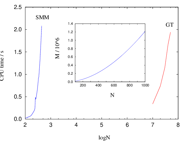

Figure 4.3:CPU time needed to calculate the total transition probabilities for a chain of length $N$ . The data is shown for a sparse-optimised matrix multiplication (SMM) method (blue) and a sparse-optimised version of Algorithm B.1 (red). Terminal nodes of each chain were connected to a sink, one of the terminal nodes was chosen to be the source. All the branching probabilities were set to $0.5$ . Each SMM calculation was terminated when $1.0 - Σ_{0}^{C_{N}}$ was less than $1 0^{- 5}$ . The inset shows the number of matrix multiplications, $M$ , as a function of chain length. Note the log $_{10}$ scale on the horizontal axes.

Mean escape times for $C_{3}$ are readily obtained from the results in Equation 4.24 by applying the method outlined in Section 4.1.5:

\begin{matrix} 𝒯_{1}^{C_{3}} & = & \frac{τ_{1} (1 - 𝒲_{2, 3, 2}) + τ_{2} P_{2, 1} + τ_{3} 𝒲_{3, 2, 1}}{1 - 𝒲_{1, 2, 1} - 𝒲_{2, 3, 2}}, \\ 𝒯_{2}^{C_{3}} & = & \frac{τ_{1} P_{1, 2} + τ_{2} + τ_{3} P_{3, 2}}{1 - 𝒲_{1, 2, 1} - 𝒲_{2, 3, 2}}, \end{matrix}

(4.29)

and $𝒯_{3}^{C_{3}}$ can be obtained from $𝒯_{1}^{C_{3}}$ by permuting the subscripts 1 and 3.

The mean escape time from the $C_{N}$ graph if started from node $β$ can be calculated recursively using the results of Appendix D and Section 4.1.5 or by resorting to a first-step analysis [241].

4.3 Complete Graphs

In a complete digraph each pair of nodes is connected by two oppositely directed edges [155]. The complete graph with $N$ graph nodes is denoted $K_{N} = (V, E)$ , and has $N$ nodes and $N (N - 1)$ edges, remembering that we have two edges per connection (Figure 4.4).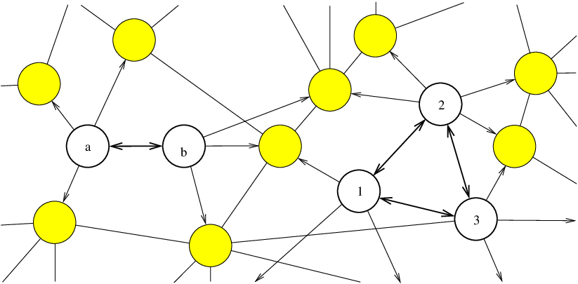

Figure 4.4:Complete graphs $K_{2}$ and $K_{3}$ , depicted as the subgraphs of a larger graph. Visible sink nodes are shaded.

Due to the complete connectivity we need only consider two cases: when the starting and finishing nodes are the same and when they are distinct. We employ complete graphs for the purposes of generality. An arbitrary graph $G_{N}$ is a subgraph of $K_{N}$ with transition probabilities for non-existent edges set to zero. All the results in this section are therefore equally applicable to arbitrary graphs.

The complete graph $K_{2}$ will not be considered here as it is topologically identical to the graph $C_{2}$ . The difference between the $K_{3}$ and $C_{3}$ graphs is the existence of edges that connect nodes $1$ and $3$ . Pathways confined to $K_{3}$ can therefore contain cycles, and for a given path length they are significantly more numerous (Figure 4.5).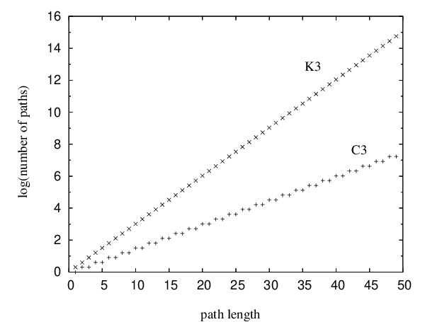

Figure 4.5:The growth of the number of pathways with the pathway length for $K_{3}$ and $C_{3}$ . The starting node is chosen arbitrarily for $K_{3}$ while for $C_{3}$ the we start at one of the terminal nodes. Any node adjacent to $K_{3}$ or $C_{3}$ is a considered to be a sink and for simplicity we consider only one escape route from every node. Note the log $_{10}$ scale on the vertical axis.

The $𝒮_{α, β}^{K_{3}}$ can again be derived analytically for this graph:

\begin{matrix} 𝒮_{1, 1}^{K_{3}} & = & \sum_{n = 0}^{\infty} {𝒲_{1, 2, 1} + 𝒲_{1, 3, 1} + 𝒲_{1, 2, 3, 1} + 𝒲_{1, 3, 2, 1}) \sum_{m = 0}^{\infty} {𝒲_{2, 3, 2})}^{m})}^{n} \\ = & \frac{1 - 𝒲_{2, 3, 2}}{1 - 𝒲_{1, 2, 1} - 𝒲_{2, 3, 2} - 𝒲_{1, 3, 1} - 𝒲_{1, 2, 3, 1} - 𝒲_{1, 3, 2, 1}}, \\ 𝒮_{2, 1}^{K_{3}} & = & \sum_{n = 0}^{\infty} {𝒲_{2, 3, 2})}^{n} P_{2, 1} + 𝒲_{2, 3, 1}) 𝒮_{1, 1}^{K_{3}} \\ = & \frac{P_{2, 1} + 𝒲_{2, 3, 1}}{1 - 𝒲_{1, 2, 1} - 𝒲_{2, 3, 2} - 𝒲_{1, 3, 1} - 𝒲_{1, 2, 3, 1} - 𝒲_{1, 3, 2, 1}} . \end{matrix}

(4.30)

The results for any other possibility can be obtained by permuting the node indices appropriately.

The pathway sums $𝒮_{α, β}^{K_{N}}$ for larger complete graphs can be obtained by recursion. For $𝒮_{N, N}^{K_{N}}$ any path leaving from and returning to $N$ can be broken down into a step out of $N$ to any $i < N$ , all possible paths between $i$ and $j < N - 1$ within $K_{N - 1}$ , and finally a step back to $N$ from $j$ . All such paths can be combined together in any order, so we have a multinomial distribution [242]:

\begin{matrix} 𝒮_{N, N}^{K_{N}} & = & \sum_{n = 0}^{\infty} {\sum_{i = 1}^{N - 1} \sum_{j = 1}^{N - 1} P_{N, j} 𝒮_{j, i}^{K_{N - 1}} P_{i, N})))}^{n} \\ = & {1 - \sum_{i = 1}^{N - 1} \sum_{j = 1}^{N - 1} P_{N, j} 𝒮_{j, i}^{K_{N - 1}} P_{i, N})}^{- 1} . \end{matrix}

(4.31)

To evaluate $𝒮_{1, N}^{K_{N}}$ we break down the sum into all paths that depart from and return to $N$ , followed by all paths that leave node $N$ and reach node 1 without returning to $N$ . The first contribution corresponds to a factor of $𝒮_{N, N}^{K_{N}}$ , and the second produces a factor $P_{i, N} 𝒮_{1, i}^{K_{N - 1}}$ for every $i < N$ :

𝒮_{1, N}^{K_{N}} = 𝒮_{N, N}^{K_{N}} \sum_{i = 1}^{N - 1} 𝒮_{1, i}^{K_{N - 1}} P_{i, N},

(4.32)

where $𝒮_{1, 1}^{K_{1}}$ is defined to be unity. Any other $𝒮_{α, β}^{K_{N}}$ can be obtained by a permutation of node labels.

Algorithm B.2 provides an example implementation of the above formulae optimised for incomplete graphs. The running time of Algorithm B.2 depends strongly on the graph density. (A digraph in which the number of edges is close to the maximum value of $N (N - 1)$ is termed a dense digraph [202].) For $K_{N}$ the algorithm runs in $𝒪 (N^{2 N})$ time, while for an arbitrary graph it scales as $𝒪 (d^{2 N})$ , where $d$ is the average degree of the nodes. For chain graphs the algorithm runs in $𝒪 (N)$ time and therefore constitutes a recursive-function-based alternative to Algorithm B.1 with linear memory requirements. For complete graphs an alternative implementation with $𝒪 ({(N!)}^{2})$ scaling is also possible.

Although the scaling of the above algorithm with $N$ may appear disastrous, it does in fact run faster than standard KMC and MM approaches for graphs where the escape probabilities are several orders of magnitude smaller than the transition probabilities (Algorithm B.2). Otherwise, for anything but moderately branched chain graphs, Algorithm B.2 is significantly more expensive. However, the graph-transformation-based method presented in Section 4.4 yields both the pathway sums and the mean escape times for a complete graph $K_{N}$ in $𝒪 (N^{3})$ time, and is the fastest approach that we have found.

Mean escape times for $K_{3}$ are readily obtained from the results in Equation 4.30 by applying the method outlined in Section 4.1.5:

𝒯_{1}^{K_{3}} = \frac{τ_{1} (1 - 𝒲_{2, 3, 2}) + τ_{2} (P_{2, 1} + 𝒲_{2, 3, 1}) + τ_{3} (P_{3, 1} + 𝒲_{3, 2, 1})}{1 - 𝒲_{1, 2, 1} - 𝒲_{2, 3, 2} - 𝒲_{3, 1, 3} - 𝒲_{1, 2, 3, 1} - 𝒲_{1, 3, 2, 1}} .

(4.33)

We have verified this result analytically using first-step analysis and numerically for various values of the parameters $τ_{i}$ and $P_{α, β}$ . and obtained quantitative agreement (see Figure 4.6).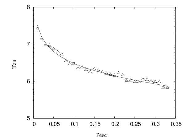

Figure 4.6:Mean escape time from $K_{3}$ as a function of the escape probability $ℰ$ . The transition probabilities for the $K_{3}$ graph are parametrised by $ℰ$ for simplicity: $P_{i, j} = (1 - ℰ) ∕ 2$ for all $i, j \in {1, 2, 3}$ and $ℰ_{1} = ℰ_{2} = ℰ_{3} = ℰ$ . Kinetic Monte Carlo data (triangles) was obtained by averaging over $100$ trajectories for each of 33 parameterisations. The solid line is the exact solution obtained using Equation 4.33. The units of $𝒯^{K_{3}}$ are arbitrary. Note the log $_{10}$ scale on the vertical axis.

Figure 4.7 demonstrates how the advantage of exact summation over KMC and MM becomes more pronounced as the escape probabilities become smaller.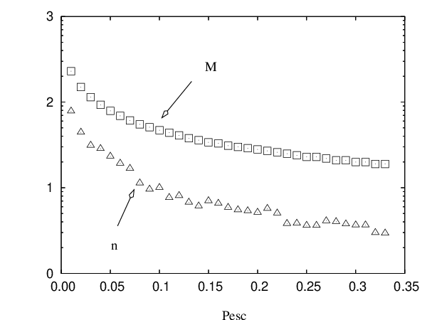

Figure 4.7:The computational cost of the kinetic Monte Carlo and matrix multiplication methods as a function of escape probability for $K_{3}$ (see caption to Figure 4.6 for the definition of $ℰ$ ). $M$ is the number of matrix multiplications required to converge the value of the total probability of getting from node $1$ to nodes $1$ , $2$ and $3$ : the calculation was terminated when the change in the total probability between iterations was less than $1 0^{- 3}$ . The number of matrix multiplications $M$ and the average trajectory length $l>$ can be used as a measure of the computational cost of the matrix multiplication and kinetic Monte Carlo approaches, respectively. The computational requirements of the exact summation method are independent of $ℰ$ . Note the log $_{10}$ scale on the vertical axis.

4.4 Graph Transformation Method

The problem of calculation of the properties of a random walk on irregular networks was addressed previously by Goldhirsch and Gefen [208, 209]. They described a generating-function-based method where an ensemble of pathways is partitioned into ‘basic walks’. A walk was defined as a set of paths that satisfies a certain restriction. As the probability generating functions corresponding to these basic walks multiply, the properties of a network as a whole can be inferred given knowledge of the generating functions corresponding to these basic walks. The method was applied to a chain, a loopless regularly branched chain and a chain containing a single loop. To the best of our knowledge only one [243] out of the 30 papers [209–211, 219–222, 240, 243–264] that cite the work of Goldhirsch and Gefen [208] is an application, perhaps due to the complexity of the method.

Here we present a graph transformation (GT) approach for calculating the pathway sums and the mean escape times for $K_{N}$ . In general, it is applicable to arbitrary digraphs, but the best performance is achieved when the graph in question is dense. The algorithm discussed in this section will be referred to as DGT (D for dense). A sparse-optimised version of the GT method (SGT) will be discussed in Section 4.5.

The GT approach is similar in spirit to the ideas that lie behind the mean value analysis and aggregation/disaggregation techniques commonly used in the performance and reliability evaluation of queueing networks [187, 265–267]. It is also loosely related to dynamic graph algorithms [268–271], which are used when a property is calculated on a graph subject to dynamic changes, such as deletions and insertions of nodes and edges. The main idea is to progressively remove nodes from a graph whilst leaving the average properties of interest unchanged. For example, suppose we wish to remove node $x$ from graph $G$ to obtain a new graph $G^{'}$ . Here we assume that $x$ is neither source nor sink. Before node $x$ can be removed the property of interest is averaged over all the pathways that include the edges between nodes $x$ and $i \in Adj [x]$ . The averaging is performed separately for every node $i$ . Next, we will use the waiting time as an example of such a property and show that the mean first passage time in the original and transformed graphs is the same.

The theory is an extension of the results used to perform jumps to second neighbours in previous KMC simulations [8, 272]. Consider KMC trajectories that arrive at node $i$ , which is adjacent to $x$ . We wish to step directly from $i$ to any node in the set of nodes $Γ$ that are adjacent to $i$ or $x$ , excluding these two nodes themselves. To ensure that the mean first-passage times from sources to sinks calculated in $G$ and $G^{'}$ are the same we must define new branching probabilities, $P_{γ, i}^{'}$ from $i$ to all $γ \in Γ$ , along with a new waiting time for escape from $i$ , $τ_{i}^{'}$ . Here, $τ_{i}^{'}$ corresponds to the mean waiting time for escape from $i$ to any $γ \in Γ$ , while the modified branching probabilities subsume all the possible recrossings involving node $x$ that could occur in $G$ before a transition to a node in $Γ$ . Hence the new branching probabilities are:

P_{γ, i}^{'} = (P_{γ, x} P_{x, i} + P_{γ, i}) \sum_{m = 0}^{\infty} {(P_{i, x} P_{x, i})}^{m} = (P_{γ, x} P_{x, i} + P_{γ, i}) ∕ (1 - P_{i, x} P_{x, i}) .

(4.34)

This formula can also be applied if either $P_{γ, i}$ or $P_{γ, x}$ vanishes.

It is easy to show that the new branching probabilities are normalised:

\sum_{γ \in Γ} \frac{P_{γ, x} P_{x, i} + P_{γ, i}}{1 - P_{i, x} P_{x, i}} = \frac{(1 - P_{i, x}) P_{x, i} + (1 - P_{x, i})}{1 - P_{i, x} P_{x, i}} = 1 .

(4.35)

To calculate $τ_{i}^{'}$ we use the method of Section 4.1.4:

τ_{i}^{'} = {\frac{d}{dζ} \sum_{γ \in Γ} \frac{P_{γ, x} P_{x, i} e^{ζ (τ_{x} + τ_{i})} + P_{γ, i} e^{ζ τ_{i}}}{1 - P_{i, x} P_{x, i} e^{ζ (τ_{x} + τ_{i})}}]}_{ζ = 0} = \frac{τ_{i} + P_{x, i} τ_{x}}{1 - P_{i, x} P_{x, i}} .

(4.36)

The modified branching probabilities and waiting times could be used in a KMC simulation based upon graph $G^{'}$ . Here we continue to use the notation of Section 4.1.4, where sinks correspond to nodes $a \in A$ and sources to nodes in $b \in B$ , and $G$ contains all the nodes in $𝒢$ expect for the $A$ set, as before. Since the modified branching probabilities, $P_{γ, i}^{'}$ , in $G^{'}$ subsume the sums over all path paths from $i$ to $γ$ that involve $x$ we would expect the sink probability, $Σ_{a, b}^{G}$ , of a trajectory starting at $b$ ending at sink $a$ , to be conserved. However, since each trajectory exiting from $γ \in Γ$ acquires a time increment equal to the average value, $τ_{i}^{'}$ , the mean first-passage times to individual sinks, $𝒯_{a, b}^{G}$ , are not conserved in $G^{'}$ (unless there is a single sink). Nevertheless, the overall mean first-passage time to $A$ is conserved, i.e. $\sum_{a \in A} 𝒯_{a, b}^{G^{'}} = 𝒯_{b}^{G^{'}} = 𝒯_{b}^{G}$ . To prove these results more formally within the framework of complete sums consider the effect of removing node $x$ on trajectories reaching node $i \in Adj [x]$ from a source node $b$ . The sink probability for a particular sink $a$ is

\begin{matrix} Σ_{a, b}^{G} & = & \sum_{ξ \in a \leftarrow b} 𝒲_{ξ} \\ = & \sum_{ξ_{1} \in i \leftarrow b} 𝒲_{ξ_{1}} \sum_{γ \in Γ} (P_{γ, i} + P_{x, i} P_{γ, x}) \sum_{m = 0}^{\infty} {(P_{i, x} P_{x, i})}^{m} \sum_{ξ_{2} \in a \leftarrow γ} 𝒲_{ξ_{2}} \\ = & \sum_{ξ_{1} \in i \leftarrow b} 𝒲_{ξ_{1}} \sum_{γ \in Γ} P_{γ, i}^{'} \sum_{ξ_{2} \in a \leftarrow γ} 𝒲_{ξ_{2}}, \end{matrix}

(4.37)

and similarly for any other node adjacent to $x$ . Hence the transformation preserves the individual sink probabilities for any source.

Now consider the effect of removing node $x$ on the mean first-passage time from source $b$ to sink $a$ , $𝒯_{a, b}^{G^{'}}$ , using the approach of Section 4.1.4.

\begin{matrix} 𝒯_{a, b}^{G^{'}} & = & {\frac{d}{dζ} \sum_{ξ_{1} \in i \leftarrow b} {\tilde{𝒲}}_{ξ_{1}} \sum_{γ \in Γ} {\tilde{P}}_{γ, i}^{'} \sum_{ξ_{2} \in a \leftarrow γ} {\tilde{𝒲}}_{ξ_{2}}]}_{ζ = 0} \\ = & \sum_{ξ_{1} \in i \leftarrow b} {\frac{d {\tilde{𝒲}}_{ξ_{1}}}{dζ}]}_{ζ = 0} \sum_{γ \in Γ} P_{γ, i}^{'} \sum_{ξ_{2} \in a \leftarrow γ} 𝒲_{ξ_{2}} \\ + \sum_{ξ_{1} \in i \leftarrow b} 𝒲_{ξ_{1}} \sum_{γ \in Γ} {\frac{d {\tilde{P}}_{γ, i}^{'}}{dζ}]}_{ζ = 0} \sum_{ξ_{2} \in a \leftarrow γ} 𝒲_{ξ_{2}} \\ + \sum_{ξ_{1} \in i \leftarrow b} 𝒲_{ξ_{1}} \sum_{γ \in Γ} P_{γ, i}^{'} \sum_{ξ_{2} \in a \leftarrow γ} {\frac{d {\tilde{𝒲}}_{ξ_{2}}}{dζ}]}_{ζ = 0}, \end{matrix}

(4.38)

where the tildes indicate that every branching probability $P_{α, β}$ is replaced by $P_{α, β} e^{ξ τ_{β}}$ , as above. The first and last terms are unchanged from graph $G$ in this construction, but the middle term,

\begin{matrix} \sum_{ξ_{1} \in i \leftarrow b} 𝒲_{ξ_{1}} \sum_{γ \in Γ} {\frac{d {\tilde{P}}_{γ, i}^{'}}{dζ}]}_{ζ = 0} \sum_{ξ_{2} \in a \leftarrow γ} 𝒲_{ξ_{2}} \\ = & \sum_{ξ_{1} \in i \leftarrow b} 𝒲_{ξ_{1}} \sum_{γ \in Γ} \frac{P_{γ, x} P_{x, i} (τ_{i} + τ_{x}) + P_{γ, i} (τ_{i} + P_{i, x} P_{x, i} τ_{x})}{{(1 - P_{i, x} P_{x, i})}^{2}} \sum_{ξ_{2} \in a \leftarrow γ} 𝒲_{ξ_{2}}, \end{matrix}

(4.39)

is different (unless there is only one sink). However, if we sum over sinks then

\sum_{a \in A} \sum_{ξ_{2} \in a \leftarrow γ} 𝒲_{ξ_{2}} = 1

(4.40)

for all $γ$ , and we can now simplify the sum over $γ$ as

\sum_{γ \in Γ} \frac{P_{γ, x} P_{x, i} (τ_{i} + τ_{x}) + P_{γ, i} (τ_{i} + P_{i, x} P_{x, i} τ_{x})}{{(1 - P_{i, x} P_{x, i})}^{2}} = τ_{i}^{'} = \sum_{γ \in Γ} P_{γ, i}^{'} τ_{i}^{'} .

(4.41)

The same argument can be applied whenever a trajectory reaches a node adjacent to $x$ , so that $𝒯_{b}^{G} = 𝒯_{b}^{G^{'}}$ , as required.

The above procedure extends the BKL approach [190] to exclude not only the transitions from the current state into itself but also transitions involving an adjacent node $x$ . Alternatively, this method could be viewed as a coarse-graining of the Markov chain. Such coarse-graining is acceptable if the property of interest is the average of the distribution of times rather than the distribution of times itself. In our simulations the average is the only property of interest. In cases when the distribution itself is sought, the approach described here may still be useful and could be the first step in the analysis of the distribution of escape times, as it yields the exact average of the distribution.

The transformation is illustrated in Figure 4.8 for the case of a single source.

Figure 4.8:The graph transformation algorithm of Section 4.4 at work. (a) A digraph with $6$ nodes and $9$ edges. The source node is node $1$ (white), the sinks are nodes $α$ , $β$ and $γ$ (shaded), and the intermediate nodes are $2$ and $3$ (black). The waiting times and transition probabilities that parametrise the graph are given below the diagram. (b) Node $2$ and all its incoming and outgoing edges are deleted from the graph depicted in (a). Two edges $β \leftarrow 1$ and $β \leftarrow 3$ are added. The parameters for this new graph are denoted by primes and expressed in terms of the parameters for the original graph. (c) Node $3$ is now disconnected as well. The resulting graph is composed of source and sink nodes only. The total probability and waiting times coincide with these of $K_{3}$ , as expected. The new parameters are denoted by a double prime.

Figure 4.8 (a) displays the original graph and its parametrisation. During the first iteration of the algorithm node $2$ is removed to yield the graph depicted in Figure 4.8 (b). This change reduces the dimensionality of the original graph, as the new graph contains one node and three edges fewer. The result of the second, and final, iteration of the algorithm is a graph that contains source and sink nodes only, with the correct transition probabilities and mean waiting time [Figure 4.8 (c)].

We now describe algorithms to implement the above approach and calculate mean escape times from complete graphs with multiple sources and sinks. Listings for some of the algorithms discussed here are given in Appendix B. We follow the notation of Section 4.1.4 and consider a digraph $𝒢_{N}$ consisting of $N_{B}$ source nodes, $N_{A}$ sink nodes, and $N_{I}$ intervening nodes. $𝒢_{N}$ therefore contains the subgraph $G_{N_{I} + N_{B}}$ .

The result of the transformation of a graph with a single source $b$ and $N_{A}$ sinks using Algorithm B.3 is the mean escape time $𝒯_{b}^{G_{N_{I} + 1}}$ and $N_{A}$ pathway probabilities $𝒫_{ξ}$ , $ξ \in A \leftarrow b$ . Solving a problem with $N_{B}$ sources is equivalent to solving $N_{B}$ single source problems. For example, if there are two sources $b_{1}$ and $b_{2}$ we first solve a problem where only node $b_{1}$ is set to be the source to obtain $𝒯_{b_{1}}^{G_{N_{I} + N_{B}}}$ and the pathway sums from $b_{1}$ to every sink node $a \in A$ . The same procedure is then followed for $b_{2}$ .

The form of the transition probability matrix $P$ is illustrated below at three stages: first for the original graph, then at the stage when all the intervening nodes have been removed (line 16 in Algorithm B.3), and finally at the end of the procedure:

\begin{matrix} 0 & A \leftarrow I & A \leftarrow B \\ ̲ & ̲ & ̲ \\ 0 & I ⇆ I & I \leftarrow B \\ ̲ & ̲ & ̲ \\ 0 & B \leftarrow I & B ⇆ B \end{matrix}) \to \begin{matrix} 0 & 0 & A \leftarrow B \\ ̲ & ̲ & ̲ \\ 0 & 0 & 0 \\ ̲ & ̲ & ̲ \\ 0 & 0 & B ⇆ B \end{matrix}) \to \begin{matrix} 0 & 0 & A \leftarrow B \\ ̲ & ̲ & ̲ \\ 0 & 0 & 0 \\ ̲ & ̲ & ̲ \\ 0 & 0 & 0 \end{matrix}),

(4.42)

Each matrix is split into blocks that specify the transitions between the nodes of a particular type, as labelled. Upon termination, every element in the top right block of matrix $P$ is non-zero.

Algorithm B.3 uses the adjacency matrix representation of graph $𝒢_{N}$ , for which the average of the distribution of mean first passage times is to be obtained. For efficiency, when constructing the transition probability matrix $P$ we order the nodes with the sink nodes first and the source nodes last. Algorithm B.3 is composed of two parts. The first part (lines 1-16) iteratively removes all the intermediate nodes from graph $𝒢_{N}$ to yield a graph that is composed of sink nodes and source nodes only. The second part (lines 17-34) disconnects the source nodes from each other to produce a graph with $N_{A} + N_{B}$ nodes and ${(N_{A} + N_{B})}^{2}$ directed edges connecting each source with every sink. Lines 13-15 are not required for obtaining the correct answer, but the final transition probability matrix looks neater.

The computational complexity of lines 1-16 of Algorithm B.3 is $𝒪 (N_{I}^{3} + N_{I}^{2} N_{B} + N_{I}^{2} N_{A} + N_{I} N_{B}^{2} + N_{I} N_{B} N_{A})$ . The second part of Algorithm B.3 (lines 17-34) scales as $𝒪 (N_{B}^{3} + N_{B}^{2} N_{A})$ . The total complexity for the case of a single source and for the case when there are no intermediate nodes is $𝒪 (N_{I}^{3} + N_{I}^{2} N_{A})$ and $𝒪 (N_{B}^{3} + N_{B}^{2} N_{A})$ , respectively. The storage requirements of Algorithm B.3 scale as $𝒪 {(N_{I} + N_{B})}^{2})$ .

We have implemented the algorithm in Fortran 95 and timed it for complete graphs of different sizes. The results presented in Figure 4.9 confirm the overall cubic scaling. The program is GPL-licensed [273] and available online [274]. These and other benchmarks presented in this chapter were obtained for a single Intel $^{®}$ Pentium $^{®}$ 4 3.00GHz 512Kb cache processor running under the Debian GNU/Linux operating system [275]. The code was compiled and optimised using the Intel $^{®}$ Fortran compiler for Linux.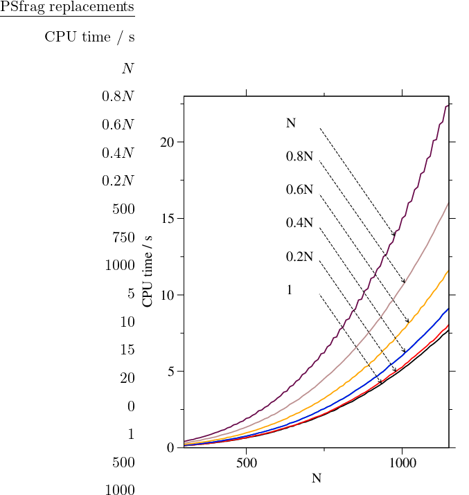

Figure 4.9:CPU time needed to transform a dense graph $G_{2 N}$ using Algorithm B.3 as a function of $N$ . The graph $G_{2 N}$ is composed of a $K_{N}$ subgraph and $N$ sink nodes. The data is shown for six different cases, when there was a single source, and when the sources comprised 20, 40, 60, 90, and 100 percent of the number of nodes in $K_{N}$ , as labelled. The data for the cases $1$ and $N$ was fitted as $5.1 \times 1 0^{- 9} N^{3}$ and $1.5 \times 1 0^{- 8} N^{3}$ , respectively (curves not shown). For case $1$ only DetachNode operations were performed while for $N$ — only Disconnect.

4.5 Applications to Sparse Random Graphs

Algorithm B.3 could easily be adapted to use adjacency-lists-based data structures [154], resulting in a faster execution and lower storage requirements for sparse graphs. We have implemented [274] a sparse-optimised version of Algorithm B.3 because the graph representations of the Markov chains of interest in the present work are sparse [201].

The algorithm for detaching a single intermediate node from an arbitrary graph stored in a sparse-optimised format is given in Algorithm B.4. Having chosen the node to be removed, $γ$ , all the neighbours $β \in Adj [γ]$ are analysed in turn, as follows. Lines 3-9 of Algorithm B.4 find node $γ$ in the adjacency list of node $β$ . If $β$ is not a sink, lines 11-34 are executed to modify the adjacency list of node $β$ : lines 13-14 delete node $γ$ from the adjacency list of $β$ , while lines 15-30 make all the neighbours $α \in Adj [γ] ⊖ β$ of node $γ$ the neighbours of $β$ . The symbol $⊖$ denotes the union minus the intersection of two sets, otherwise known as the symmetric difference. If the edge $β \to α$ already existed only the branching probability is changed (line 21). Otherwise, a new edge is created and the adjacency and branching probability lists are modified accordingly (line 26 and line 27, respectively). Finally, the branching probabilities of node $β$ are renormalised (lines 31-33) and the waiting time for node $β$ is increased (line 34).

Algorithm B.4 is invoked iteratively for every node that is neither a source nor a sink to yield a graph that is composed of source nodes and sink nodes only. Then the procedure described in Section 4.4 for disconnection of source nodes (lines 17-34 of Algorithm B.3) is applied to obtain the mean escape times for every source node. The sparse-optimised version of the second part of Algorithm B.3 is straightforward and is therefore omitted here for brevity.

The running time of Algorithm B.4 is $𝒪 (d_{c} \sum_{i \in Adj [c]} d_{i})$ , where $d_{k}$ is the degree of node $k$ . For the case when all the nodes in a graph have approximately the same degree, $d$ , the complexity is $𝒪 (d^{3})$ . Therefore, if there are $N$ intermediate nodes to be detached and $d$ is of the same order of magnitude as $N$ , the cost of detaching $N$ nodes is $𝒪 (N^{4})$ . The asymptotic bound is worse than that of Algorithm B.3 because of the searches through adjacency lists (lines 3-9 and lines 19-24). If $d$ is sufficiently small the algorithm based on adjacency lists is faster.

After each invocation of Algorithm B.4 the number of nodes is always decreased by one. The number of edges, however, can increase or decrease depending on the in- and out-degree of the node to be removed and the connectivity of its neighbours. If node $γ$ is not directly connected to any of the sinks, and the neighbours of node $γ$ are not connected to each other directly, the total number of edges is increased by $d_{γ} (3 - d_{γ})$ . Therefore, the number of edges decreases (by $2$ ) only when $d_{γ} \in {1, 2}$ , and the number of edges does not change if the degree is $3$ . For $d_{γ} > 3$ the number of edges increases by an amount that grows quadratically with $d_{γ}$ . The actual increase depends on how many connections already existed between the neighbours of $γ$ .

The order in which the intermediate nodes are detached does not change the final result and is unimportant if the graph is complete. For sparse graphs, however, the order can affect the running time significantly. If the degree distribution for successive graphs is sharp with the same average, $d$ , then the order in which the nodes are removed does not affect the complexity, which is $𝒪 (d^{3} N)$ . If the distributions are broad it is helpful to remove the nodes with smaller degrees first. A Fibonacci heap min-priority queue [276] was successfully used to achieve this result. The overhead for maintaining a heap is $d_{γ}$ increase-key operations (of $𝒪 (\log (N))$ each) per execution of Algorithm B.4. Fortran and Python implementations of Algorithm B.4 algorithm are available online [274].

Random graphs provide an ideal testbed for the GT algorithm by providing control over the graph density. A random graph, $R_{N}$ , is obtained by starting with a set of $N$ nodes and adding edges between them at random [33]. In this work we used a random graph model where each edge is chosen independently with probability $d> ∕ (N - 1)$ , where $d>$ is the target value for the average degree.

The complexity for removal of $N$ nodes can then be expressed as

𝒪 \log (N) \sum_{i \in {1, 2, 3, \dots, N}} d_{c (i)}^{2} \sum_{j \in Adj [c (i)]} d_{j, c (i)})),

(4.43)

where $d_{c (i)}$ is the degree of the node, $c (i)$ , removed at iteration $i$ , $Adj [c (i)]$ is its adjacency list, and $d_{j, c (i)}$ is the degree of the $j$ th neighbour of that node at iteration $i$ . The computational cost given in Equation 4.43 is difficult to express in terms of the parameters of the original graph, as the cost of every cycle depends on the distribution of degrees, the evolution of which, in turn, is dependent on the connectivity of the original graph in a non-trivial manner (see Figure 4.10). The storage requirements of a sparse-optimised version of GT algorithm scale linearly with the number of edges.

Figure 4.10:Evolution of the distribution of degrees for random graphs of different expected degree, $d> = 5, 10, 15$ , as labelled. This is a colour-coded projection of the probability mass function [277, 278], $P (d)$ , of the distribution of degrees as a function of the number of the detached intermediate nodes, $n$ . The straight line shows $P (d, n)$ for complete graph $K_{1000}$ . All four graphs contain a single source, 999 intermediate nodes and a single sink. The transformation was done using sparse-optimised version of Algorithm B.3 with Fibonacci-heap-based min-priority queue. It can be seen that as the intermediate nodes are detached the density of the graph that is being transformed grows. The expected degree of the initial graph determines how soon the maximum density will be reached.

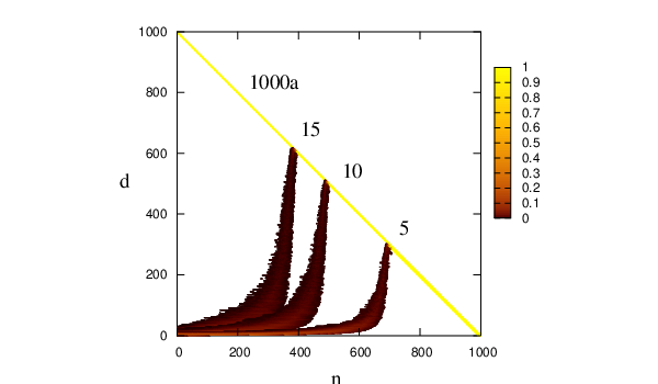
To investigate the dependence of the cost of the GT method on the number of nodes, $N$ , we have tested it on a series of random graphs $R_{N}$ for different values of $N$ and fixed average degree, $d>$ . The results for three different values of $d>$ are shown in Figure 4.11. The motivation for choosing $d>$ from the interval $3, 5]$ was the fact that most of our stationary point databases have average connectivities for the local minima that fall into this range.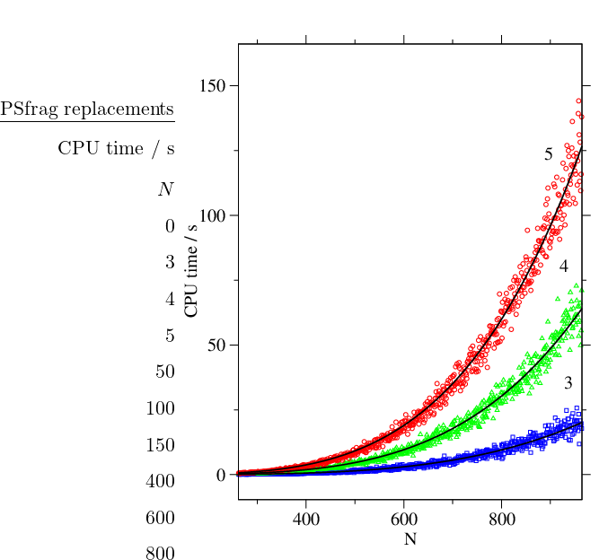

Figure 4.11:CPU time needed to transform a sparse random graph $R_{2 N}$ using the GT approach described in Section 4.4 as a function of the number of intermediate nodes, $N$ . $R_{2 N}$ is composed of a single source node, $N$ sink nodes and $N - 1$ intermediate nodes. For each value of $N$ the data for three different values of the expected degree, $d> = 3, 4, 5$ , is shown, as labelled. Solid lines are analytic fits of the form $c N^{4}$ , where $c = 2.3 \times 1 0^{- 11}, 7.4 \times 1 0^{- 11}, 1.5 \times 1 0^{- 10}$ for $d> = 3, 4, 5$ , respectively. CPU time is in seconds.

It can be seen from Figure 4.11 that for sparse random graphs $R_{N}$ the cost scales as $𝒪 (N^{4})$ with a small $d>$ -dependent prefactor. The dependence of the computational complexity on $d>$ is illustrated in Figure 4.12.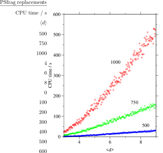

Figure 4.12:CPU time needed to transform a sparse random graph $R_{2 N}$ using the GT approach as a function of the expected degree, $d>$ . The data is shown for three graphs with $N = 500$ , $750$ and $1000$ , as labelled. $R_{2 N}$ is composed of a single source node, $N$ sink nodes and $N - 1$ intermediate nodes.

From Figure 4.10 it is apparent that at some point during the execution of the GT algorithm the graph reaches its maximum possible density. Once the graph is close to complete it is no longer efficient to employ a sparse-optimised algorithm. The most efficient approach we have found for sparse graphs is to use the sparse-optimised GT algorithm until the graph is dense enough, and then switch to Algorithm B.3. We will refer to this approach as SDGT. The change of data structures constitutes a negligible fraction of the total execution time. Figure 4.13 depicts the dependence of the CPU time as a function of the switching parameter 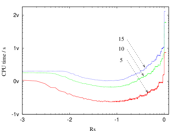$R_{s}$ .

Figure 4.13:CPU time as a function of switching ratio $R_{s}$ shown for random graphs of different expected degree, $d> = 5, 10, 15$ , as labelled. All three graphs contain a single source, 999 intermediate nodes and a single sink. The transformation was performed using the sparse-optimised version of Algorithm B.3 until the the ratio $d_{c (i)} ∕ n (i)$ became greater than $R_{s}$ . Then a partially transformed graph was converted into adjacency matrix format and the transformation was continued with Algorithm B.3. The optimal value of $R_{s}$ lies in the interval $[0.07, 0.1]$ . Note the log $_{10}$ scale on both axes.

Whenever the ratio $d_{c (i)} ∕ n (i)$ , where the $d_{c (i)}$ is the degree of intermediate node $c$ detached at iteration $i$ , and $n (i)$ is the number of the nodes on a heap at iteration $i$ , is greater than $R_{s}$ , the partially transformed graph is converted from the adjacency list format into adjacency matrix format and the transformation is continued using Algorithm B.3. It can be seen from Figure 4.10 that for the case of a random graphs with a single sink, a single source and 999 intermediate nodes the optimal values of $R_{s}$ lie in the interval $[0.07, 0.1]$ .

4.6 Overlapping Sets of Sources and Sinks

We now return to the digraph representation of a Markov chain that corresponds to the DPS pathway ensemble discussed in Section 4.1.4. A problem with (partially) overlapping sets of sources and sinks can easily be converted into an equivalent problem where there is no overlap, and then the GT method discussed in Section 4.4 and Section 4.5 can be applied as normal.

As discussed above, solving a problem with $n$ sources reduces to solving $n$ single-source problems. We can therefore explain how to deal with a problem of overlapping sets of sinks and sources for a simple example where there is a single source-sink $i$ and, optionally, a number of sink nodes.

First, a new node $i^{'}$ is added to the set of sinks and its adjacency lists are initialised to $AdjOut [i^{'}] = \emptyset$ and $AdjIn [i^{'}] = AdjIn [i]$ . Then, for every node $j \in AdjOut [i]$ we update its waiting time as $τ_{j} = τ_{j} + τ_{i}$ and add node $j$ to the set of sources with probabilistic weight initialised to $P_{j, i} W_{i}$ , where $W_{i}$ is the original probabilistic weight of source $i$ (the probability of choosing source $i$ from the set of sources). Afterwards, the node $i$ is deleted.

4.7 Applications to Lennard-Jones Clusters

4.7.1 $O_{h} \leftrightarrow I_{h}$ Isomerisation of LJ $_{38}$

We have applied the GT method to study the temperature dependence of the rate of $O_{h} \leftrightarrow I_{h}$ interconversion of 38-atom Lennard-Jones cluster. The PES sample was taken from a previous study [8] and contained 1740 minima and 2072 transition states. Only geometrically distinct structures were considered when generating this sample because this way the dimensionality of the problem is reduced approximately by a factor of $2 N! ∕ h$ , where $h$ is the order of the point group. Initial and final states in this sample roughly correspond to icosahedral-like and octahedral-like structures on the PES of this cluster. The assignment was made in Reference [8] by solving master equation numerically to find the eigenvector that corresponds to the smallest non-zero eigenvalue. As simple two-state dynamics are associated with exponential rise and decay of occupation probabilities there must exist a time scale on which all the exponential contributions to the solution of the master equation decay to zero except for the slowest [9]. The sign of the components of the eigenvector corresponding to the slowest mode was used to classify the minima as $I_{h}$ or $O_{h}$ in character [8].

The above sample was pruned to ensure that every minimum is reachable from any other minimum to create a digraph representation that contained 759 nodes including 43 source nodes and 5 sink nodes, and 2639 edges. The minimal, average and maximal degree for this graph were 2, $3.8$ and 84, respectively, and the graph density was $4.6 \times 1 0^{- 3}$ . We have used the SDGT algorithm with the switching ratio set to $0.08$ to transform this graph for several values of temperature. In each of these calculations 622 out of 711 intermediate nodes were detached using SGT, and the remaining 89 intermediate nodes were detached using the GT algorithm optimised for dense graphs (DGT).

An Arrhenius plot depicting the dependence of the rate constant on temperature is shown in Figure 4.14 (a). The running time of SDGT algorithm was $1.8 \times 1 0^{- 2}$ seconds [this value was obtained by averaging over 10 runs and was the same for each SDGT run in Figure 4.14 (a)]. For comparison, the timings obtained using the SGT and DGT algorithms for the same problem were $2.0 \times 1 0^{- 2}$ and $89.0 \times 1 0^{- 2}$ seconds, respectively. None of the 43 total escape probabilities (one for every source) deviated from unity by more than $1 0^{- 5}$ for temperatures above $T = 0.07$ (reduced units). For lower temperatures the probability was not conserved due to numerical imprecision.

The data obtained using SDGT method is compared with results from KMC simulation, which require increasingly more CPU time as the temperature is lowered. Figure 4.14 also shows the data for KMC simulations at temperatures $0.14$ , $0.15$ , $0.16$ , $0.17$ and $0.18$ . Each KMC simulation consisted of the generation of an ensemble of 1000 KMC trajectories from which the averages were computed. The cost of each KMC calculation is proportional to the average trajectory length, which is depicted in Figure 4.14 (b) as a function of the inverse temperature. The CPU timings for each of these calculations were (in the order of increasing temperature, averaged over five randomly seeded KMC simulations): $125$ , $40$ , $18$ , $12$ , and $7$ seconds. It can be seen that using GT method we were able to obtain kinetic data for a wider range of temperatures and with less computational expense.

Figure 4.14:(a) Arrhenius plots for the LJ $_{38}$ cluster. $k$ is the rate constant corresponding to transitions from icosahedral-like to octahedral-like regions. Green circles represent the data obtained from 23 SDGT runs at temperatures $T \in {0.07, 0.075, \dots, 0.18}$ . The data from five KMC runs is also shown (red squares). The data shown in blue corresponds to temperatures $T \in {0.035, 0.04, \dots, 0.065}$ and was obtained using the SDGT2 method (discussed in Section 4.7.2) with quadruple precision enabled. In all SDGT runs the total escape probabilities calculated for every source at the end of the calculation deviated from unity by no more then $1 0^{- 5}$ . For this PES sample the lowest temperature for which data was reported in previous works was $T = 0.08$ . (b) The average KMC trajectory length [data in direct correspondence with KMC results shown in (a)]. A solid line is used to connect the data points to guide the eye.

4.7.2 Internal Diffusion in LJ $_{55}$

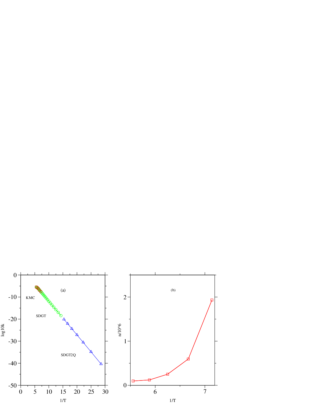
We have applied the graph transformation method to study the centre-to-surface atom migration in 55-atom Lennard-Jones cluster. The global potential energy minimum for LJ $_{55}$ is a Mackay icosahedron, which exhibits special stability and ‘magic number’ properties [279, 280]. Centre-to-surface and surface-to-centre rates of migration of a tagged atom for this system were considered in previous work [10]. In Reference [10] the standard DPS procedure was applied to create and converge an ensemble of paths linking the structure of the global minimum with the tagged atom occupying the central position and structures where tagged atom is placed in sites that lie on fivefold and twofold symmetry axes (Figure 4.15). We have reused this sample in the present work.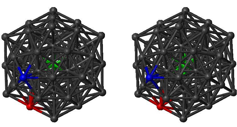

Figure 4.15:Global minimum of the LJ $_{55}$ cluster (shown in stereo). The tagged atom can occupy the central position (green) or one of the two different surface sites (red and blue).

The sample contained 9907 minima and 19384 transition states. We excluded transition states that facilitate degenerate rearrangements from consideration. For minima interconnected by more than one transition state we added the rate constants in each direction to calculate the branching probabilities. Four digraph representations were created with minimum degrees of 1, 2, 3 and 4 via iterative removal of the nodes with degrees that did not satisfy the requirement. These digraphs will be referred to as digraphs 1, 2, 3 and 4, respectively. The corresponding parameters are summarised in Table 4.1. Since the cost of the GT method does not depend on temperature we also quote CPU timings for the DGT, SGT and SDGT methods for each of these graphs in the last three columns of Table 4.1. Each digraph contained two source nodes labelled $1$ and $2$ and a single sink. The sink node corresponds to the global minimum with the tagged atom in the centre (Figure 4.15). It is noteworthy that the densities of the graphs corresponding to both our samples (LJ $_{38}$ and LJ $_{55}$ ) are significantly lower than the values predicted for a complete sample [115], which makes the use of sparse-optimised methods even more advantageous. From Table 4.1 it is clear that the SDGT approach is the fastest, as expected; we will use SDGT for all the rate calculations in the rest of this section.

Table 4.1:Properties of four digraphs corresponding to the LJ

_{55}

PES sample from an internal diffusion study.

| V |

is the number of nodes;

| E |

is the number of directed edges;

d_{\min}

d>

and

d_{\max}

are the minimum, average and maximum degrees, respectively;

ρ

is the graph density, defined as a ratio of the number of edges to the maximum possible number of edges;

r

and

d

are the graph radius and diameter, defined as the maximum and minimum node eccentricity, respectively, where the eccentricity of a node

v

is defined as the maximum distance between

v

and any other node.

l>

is the average distance between nodes. The CPU time,

t

, necessary to transform each graph using the DGT, SGT and SDGT methods is given in seconds for a single 32-bit Intel

^{®}

Pentium

^{®}

4 3.00 GHz 512 Kb cache processor.



$\| V \|$	$\| E \|$	$d_{\min}$	$d>$		$d_{\max}$	$ρ ∕ 1 0^{- 4}$		$r$	$l>$		$d$	$t_{DGT}$		$t_{SGT}$		$t_{SDGT}$

9843	34871	1	3.	9	983	3.	6	10	5.	71	20	2346.	1	39.	6	1.	36
6603	28392	2	4.	8	983	6.	5	9	4.	86	17	1016.	1	38.	9	1.	33
2192	14172	3	7.	9	873	29.	5	4	3.	63	8	46.	9	5.	9	0.	49
865	7552	4	1.	9	680	101.	0	4	3.	07	7	3.	1	0.	8	0.	12

For this sample KMC calculations are unfeasible at temperatures lower than about $T = 0.3$ (Here $T$ is expressed in the units of $𝜖 ∕ k_{B}$ ). Already for $T = 0.4$ the average KMC trajectory length is $7.5 \times 1 0^{6}$ (value obtained by averaging over 100 trajectories). In previous work it was therefore necessary to use the DPS formalism, which invokes a steady-state approximation for the intervening minima, to calculate the rate constant at temperatures below $0.35$ [10]. Here we report results that are in direct correspondence with the KMC formulation of the problem, for temperatures as low as $0.1$ .

Figure 4.16 presents Arrhenius plots that we calculated using the SDGT method for this system. The points in the green dataset are the results from seven SDGT calculations at temperatures $T \in {0.3, 0.35, \dots, 0.6}$ conducted for each of the digraphs. The total escape probabilities, $Σ_{1}^{G}$ and $Σ_{2}^{G}$ , calculated for each of the two sources at the end of the calculation deviated from unity by no more than $1 0^{- 5}$ . For higher temperatures and smaller digraphs the deviation was smaller, being on the order of $1 0^{- 10}$ for digraph 4 at $T = 0.4$ , and improving at higher temperatures and/or smaller graph sizes.

At temperatures lower than $0.3$ the probability deviated by more than $1 0^{- 5}$ due to numerical imprecision. This problem was partially caused by the round-off errors in evaluation of terms $1 - P_{α, β} P_{β, α}$ , which increase when $P_{α, β} P_{β, α}$ approaches unity. These errors can propagate and amplify as the evaluation proceeds. By writing

\begin{matrix} P_{α, β} & = & 1 - \sum_{γ \neq α} P_{γ, β} \equiv 1 - 𝜖_{α, β} \\ and P_{β, α} & = & 1 - \sum_{γ \neq β} P_{γ, α} \equiv 1 - 𝜖_{β, α}, \end{matrix}

(4.44)

and then using

1 - P_{α, β} P_{β, α} = 𝜖_{α, β} - 𝜖_{α, β} 𝜖_{β, α} + 𝜖_{β, α}

(4.45)

we were able to decrease $1 - Σ_{α}^{G}$ by several orders of magnitude at the expense of doubling the computational cost. The SDGT method with probability denominators evaluated in this fashion will be referred to as SDGT1.

Terms of the form $1 - P_{α, β} P_{β, α}$ approach zero when nodes $α$ and $β$ become ‘effectively’ (i.e. within available precision) disconnected from the rest of the graph. If this condition is encountered in the intermediate stages of the calculation it could also mean that a larger subgraph of the original graph is effectively disconnected. The waiting time for escape if started from a node that belongs to this subgraph tends to infinity. If the probability of getting to such a node from any of the source nodes is close to zero the final answer may still fit into available precision, even though some of the intermediate values cannot. Obtaining the final answer in such cases can be problematic as division-by-zero exceptions may occur.

Another way to alleviate numerical problems at low temperatures is to stop round-off errors from propagation at early stages by renormalising the branching probabilities of affected nodes $β \in Adj [γ]$ after node $γ$ is detached. The corresponding check that the updated probabilities of node $β$ add up to unity could be inserted after line 33 of Algorithm B.4 (see Appendix B), and similarly for Algorithm B.3. A version of SDGT method with this modification will be referred to as SDGT2.

Both SDGT1 and SDGT2 have similarly scaling overheads relative to the SDGT method. We did not find any evidence for superiority of one scheme over another. For example, the SDGT calculation performed for digraph 4 at $T = 0.2$ yielded $𝒯^{G} = 𝒯_{1}^{G} W_{1} + 𝒯_{2}^{G} W_{2} = 6.4 \times 1 0^{- 18}$ , and precision was lost as both $Σ_{1}^{G}$ and $Σ_{2}^{G}$ were less than $1 0^{- 5}$ . The SDGT1 calculation resulted in $𝒯^{G} = 8.7 \times 1 0^{- 22}$ and $Σ_{1}^{G} = Σ_{2}^{G} = 1.0428$ , while the SDGT2 calculation produced $𝒯^{G} = 8.4 \times 1 0^{- 22}$ with $Σ_{1}^{G} = Σ_{2}^{G} = 0.99961$ . The CPU time required to transform this graph using our implementations of the SDGT1 and SDGT2 methods was $0.76$ and $0.77$ seconds, respectively.

To calculate the rates at temperatures in the interval $[0.1, 0.3]$ reliably we used an implementation of the SDGT2 method compiled with quadruple precision (SDGT2Q) (note that the architecture is the same as in other benchmarks, i.e. with 32 bit wide registers). The points in the blue dataset in Figure 4.16 are the results from 4 SDGT2Q calculations at temperatures 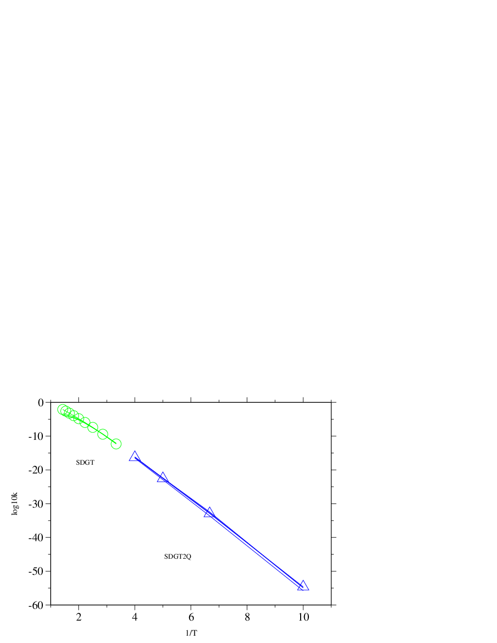$T \in {0.10, 0.35, \dots, 0.75}$ .

Figure 4.16:Arrhenius plots for four digraphs of varying sizes (see Table 4.1) created from a sample of the PES for the LJ $_{55}$ cluster. $k$ is the rate constant corresponding to surface-to-centre migration of a tagged atom. Calculations were conducted at $T \in {0.3, 0.35, \dots, 0.7}$ using the SDGT method (green) and $T \in {0.1, 0.15, \dots, 0.25}$ using SDGT2Q (blue). For each of the digraphs the calculations yielded essentially identical results so data points for only one of them are shown.

By using SDGT2Q we were also able to improve on the low-temperature results for LJ $_{38}$ presented in the previous section. The corresponding data is shown in blue in Figure 4.14.

4.8 Summary

The most important result of this chapter is probably the graph transformation (GT) method. The method works with a digraph representation of a Markov chain and can be used to calculate the first moment of a distribution of the first-passage times, as well as the total transition probabilities for an arbitrary digraph with sets of sources and sinks that can overlap. The calculation is performed in a non-iterative and non-stochastic manner, and the number of operations is independent of the simulation temperature.

We have presented three implementations of the GT algorithm: sparse-optimised (SGT), dense-optimised (DGT), and hybrid (SDGT), which is a combination of the first two. The SGT method uses a Fibonacci heap min-priority queue to determine the order in which the intermediate nodes are detached to achieve slower growth of the graph density and, consequently, better performance. SDGT is identical to DGT if the graph is dense. For sparse graphs SDGT performs better then SGT because it switches to DGT when the density of a graph being transformed approaches the maximum. We find that for SDGT method performs well both for sparse and dense graphs. The worst case asymptotic scaling of SDGT is cubic.

We have also suggested two versions of the SDGT method that can be used in calculations where a greater degree of precision is required. The code that implements SGT, DGT, SDGT, SDGT1 and SDGT2 methods is available for download [274].

The connection between the DPS and KMC approaches was discussed in terms of digraph representations of Markov chains. We showed that rate constants obtained using the KMC or DPS methods can be computed using graph transformation. We have presented applications to the isomerisation of the LJ $_{38}$ cluster and the internal diffusion in the LJ $_{55}$ cluster. Using the GT method we were able to calculate rate constants at lower temperatures than was previously possible, and with less computational expense.

We also obtained analytic expressions for the total transition probabilities for arbitrary digraphs in terms of combinatorial sums over pathway ensembles. It is hoped that these results will help in further theoretical pursuits, e.g. these aimed at obtaining higher moments of the distribution of the first passage times for arbitrary Markov chains.

Finally, we showed that the recrossing contribution to the DPS rate constant of a given discrete pathway can be calculated exactly. We presented a comparison between a sparse-optimised matrix multiplication method and a sparse-optimised version of Algorithm B.1 and showed that it is beneficial to use Algorithm B.1 because it is many orders of magnitude faster, runs in linear time and has constant memory requirements.

[next] [prev] [prev-tail] [front] [up]

Chapter 4Ensembles of Rearrangement Pathways